Tobramycin serum and ELF (Van Wart 2025)
Source:vignettes/articles/VanWart_2025_tobramycin.Rmd
VanWart_2025_tobramycin.RmdModel and source
ui <- rxode2::rxode(readModelDb("VanWart_2025_tobramycin"))
#> ℹ parameter labels from comments will be replaced by 'label()'- Citation: Van Wart SA, Trang M, Safir MC, Santulli AR, Rubino CM, Bhavnani SM. Population pharmacokinetic analysis of tobramycin in serum and ELF using data from patients with pneumonia. Antimicrob Agents Chemother. 2025;69(5):e0090824. doi:10.1128/aac.00908-24. Parameter estimates are from Table 1; the structural equations, the creatinine clearance derivation, and the residual-error structure are from the NONMEM control stream printed on page 5 of the supplemental material (aac.00908-24-s0001.pdf). The underlying serum and ELF concentration data were published by Carcas AJ, Garcia-Satue JL, Zapater P, Frias-Iniesta J. Tobramycin penetration into epithelial lining fluid of patients with pneumonia. Clin Pharmacol Ther. 1999;65(3):245-250. doi:10.1016/S0009-9236(99)70103-7.
- Description: Two-compartment population PK model for tobramycin in serum with zero-order intravenous input, first-order elimination, and a linked epithelial-lining-fluid (ELF) effect compartment, developed on time-matched steady-state serum and urea-corrected ELF (bronchoalveolar-lavage) concentrations from 16 adult patients with pneumonia originally published by Carcas 1999 (Van Wart 2025). The ELF compartment is driven by the serum concentration and does not remove drug from the central compartment, so it is a partitioned effect compartment rather than a distribution compartment: the pseudo-partition coefficient ppc = k13 / k30 = 0.49 sets the steady-state ELF:serum ratio and the equilibration rate ke0 = k30 gives an equilibration half-life of about 12 minutes. Body-surface-area-normalised creatinine clearance, computed inside the model from weight, height, age, sex, and serum creatinine, acts on clearance as a power function referenced to 90 mL/min/1.73 m2. Central and peripheral volumes were constrained equal during fitting (Vss 20.8 L).
- Article: https://doi.org/10.1128/aac.00908-24
- Supplement (structural model diagram, goodness-of-fit plots, NONMEM control stream, and the complete analysis data set): https://europepmc.org/article/MED/40227040#supplementary-material
Van Wart 2025 is a re-analysis of the tobramycin serum and epithelial lining fluid (ELF) data published by Carcas 1999. Its purpose is to quantify the steady-state ELF penetration ratio for an aminoglycoside using time-staggered bronchoalveolar-lavage (BAL) sampling, so that the ELF exposure can be carried into later pharmacokinetic-pharmacodynamic target-attainment work.
Structurally the model is a two-compartment serum PK model with
zero-order intravenous input and first-order elimination, plus a third
compartment for ELF that is driven by the serum concentration
but returns nothing to it. In the paper’s own words, the model “used
serum drug concentrations to drive appearance in and subsequent removal
of drug from the ELF without impacting the serum PK data fitting”. That
makes it a partitioned effect compartment rather than a distribution
compartment, and it is encoded here in the canonical ke0 /
ppc form.
Population
The model was fit to 16 adult patients with pneumonia who underwent bronchoscopy with BAL. Each patient received tobramycin as a 30-minute intravenous infusion every 8 hours, nominally 1 mg/kg with dose adjustment as needed to reach peak and trough concentrations of approximately 8 and < 2 mg/L; bronchoscopy was performed at least 2 days after any adjustment, so serum concentrations were at steady state. Serum concentrations were measured at 0.5, 2, 4, and 8 hours after the previous dose, and a single urea-corrected ELF concentration was collected per patient at one of those four times (four patients per time point). Demographics span 23-72 years (median 43 years) and 50-84 kg (median 68 kg), with 31.2% female; the complete 16-subject analysis data set is printed on pages 7-9 of the supplemental material and is reproduced below.
str(ui$population)
#> List of 13
#>  $ species       : chr "human"
#>  $ n_subjects    : int 16
#>  $ n_studies     : int 1
#>  $ age_range     : chr "23-72 years (median 43 years)"
#>  $ weight_range  : chr "50-84 kg (median 68 kg)"
#>  $ height_range  : chr "147-190 cm"
#>  $ sex_female_pct: num 31.2
#>  $ disease_state : chr "Adults with pneumonia undergoing bronchoscopy with bronchoalveolar lavage."
#>  $ renal_function: chr "Serum creatinine 0.6-1.2 mg/dL. Derived creatinine clearance spans roughly 60-160 mL/min/1.73 m^2 using the con"| __truncated__
#>  $ dose_range    : chr "1 mg/kg tobramycin as a 30-minute IV infusion every 8 h, with dose adjustment as needed to reach peak and troug"| __truncated__
#>  $ regions       : chr "Spain (the source clinical study of Carcas 1999)."
#>  $ n_observations: chr "63 serum concentrations and 16 urea-corrected ELF concentrations (1 per patient, 4 patients at each of 0.5, 2, "| __truncated__
#>  $ notes         : chr "Van Wart 2025 is a re-analysis: it fits a population PK model to individual dosing, demographic, renal-function"| __truncated__
# The published 16-subject NONMEM analysis data set (supplemental material,
# pages 7-9). Covariates are one row per subject.
subjects <- tibble::tribble(
  ~id, ~WT, ~AGE, ~SEXF, ~HT, ~CREAT,
   1L,  73,   72,    0,  164,   0.9,
   2L,  68,   49,    0,  148,   1.0,
   3L,  68,   36,    0,  190,   1.0,
   4L,  50,   34,    1,  157,   1.0,
   5L,  71,   28,    1,  159,   0.9,
   6L,  67,   44,    1,  159,   0.6,
   7L,  65,   48,    0,  158,   1.1,
   8L,  84,   56,    1,  147,   0.6,
   9L,  77,   25,    0,  176,   1.2,
  10L,  60,   45,    1,  159,   0.7,
  11L,  62,   39,    0,  156,   1.0,
  12L,  68,   47,    0,  168,   1.0,
  13L,  59,   23,    0,  172,   0.9,
  14L,  70,   67,    0,  168,   0.7,
  15L,  67,   41,    0,  163,   0.9,
  16L,  69,   42,    0,  169,   1.1
)

# Observed steady-state concentrations, by time since last dose (TSLD).
# matrix = "Serum" for CMT 1 records and "ELF" for CMT 3 records.
observed <- tibble::tribble(
  ~id, ~tsld, ~matrix, ~dv,
   1L, 0.5, "Serum", 6.08,  1L, 2.0, "Serum", 4.57,  1L, 4.0, "Serum", 2.87,
   1L, 8.0, "Serum", 1.47,  1L, 4.0, "ELF",   3.40,
   2L, 0.5, "Serum", 8.37,  2L, 2.0, "Serum", 6.00,  2L, 4.0, "Serum", 3.29,
   2L, 8.0, "Serum", 1.16,  2L, 0.5, "ELF",   2.54,
   3L, 0.5, "Serum", 9.09,  3L, 2.0, "Serum", 4.72,  3L, 4.0, "Serum", 2.67,
   3L, 8.0, "Serum", 1.01,  3L, 0.5, "ELF",   2.57,
   4L, 0.5, "Serum", 6.42,  4L, 2.0, "Serum", 4.37,  4L, 4.0, "Serum", 2.54,
   4L, 8.0, "Serum", 0.87,  4L, 4.0, "ELF",   0.93,
   5L, 0.5, "Serum", 4.58,  5L, 2.0, "Serum", 2.57,  5L, 4.0, "Serum", 1.13,
   5L, 8.0, "Serum", 0.27,  5L, 8.0, "ELF",   0.43,
                            6L, 2.0, "Serum", 2.54,  6L, 4.0, "Serum", 1.15,
   6L, 8.0, "Serum", 0.31,  6L, 0.5, "ELF",   1.46,
   7L, 0.5, "Serum", 6.18,  7L, 2.0, "Serum", 4.36,  7L, 4.0, "Serum", 1.69,
   7L, 8.0, "Serum", 0.54,  7L, 2.0, "ELF",   2.25,
   8L, 0.5, "Serum", 7.09,  8L, 2.0, "Serum", 4.83,  8L, 4.0, "Serum", 2.32,
   8L, 8.0, "Serum", 0.61,  8L, 0.5, "ELF",   2.34,
   9L, 0.5, "Serum", 7.74,  9L, 2.0, "Serum", 5.49,  9L, 4.0, "Serum", 4.17,
   9L, 8.0, "Serum", 0.86,  9L, 2.0, "ELF",   1.56,
  10L, 0.5, "Serum", 8.47, 10L, 2.0, "Serum", 6.64, 10L, 4.0, "Serum", 2.57,
  10L, 8.0, "Serum", 1.56, 10L, 4.0, "ELF",   1.17,
  11L, 0.5, "Serum", 8.50, 11L, 2.0, "Serum", 3.98, 11L, 4.0, "Serum", 1.76,
  11L, 8.0, "Serum", 0.60, 11L, 8.0, "ELF",   0.45,
  12L, 0.5, "Serum", 8.07, 12L, 2.0, "Serum", 3.61, 12L, 4.0, "Serum", 1.82,
  12L, 8.0, "Serum", 0.48, 12L, 4.0, "ELF",   1.00,
  13L, 0.5, "Serum", 4.92, 13L, 2.0, "Serum", 2.14, 13L, 4.0, "Serum", 1.08,
  13L, 8.0, "Serum", 0.93, 13L, 8.0, "ELF",   1.15,
  14L, 0.5, "Serum", 6.63, 14L, 2.0, "Serum", 3.56, 14L, 4.0, "Serum", 2.02,
  14L, 8.0, "Serum", 0.72, 14L, 2.0, "ELF",   2.12,
  15L, 0.5, "Serum", 6.39, 15L, 2.0, "Serum", 2.71, 15L, 4.0, "Serum", 1.52,
  15L, 8.0, "Serum", 0.76, 15L, 2.0, "ELF",   0.76,
  16L, 0.5, "Serum", 4.96, 16L, 2.0, "Serum", 3.19, 16L, 4.0, "Serum", 1.66,
  16L, 8.0, "Serum", 0.41, 16L, 8.0, "ELF",   1.04
)

# Subject 6 has no 0.5 h serum sample in the published data set.
stopifnot(sum(observed$matrix == "Serum") == 63L,
          sum(observed$matrix == "ELF") == 16L)
observed %>% count(matrix, tsld) %>% tidyr::pivot_wider(names_from = matrix, values_from = n)
#> # A tibble: 4 × 3
#>    tsld   ELF Serum
#>   <dbl> <int> <int>
#> 1   0.5     4    15
#> 2   2       4    16
#> 3   4       4    16
#> 4   8       4    16
The renal-function covariate is derived inside the model rather than supplied as a column, so the derived creatinine clearance of the analysis population is worth stating explicitly.
subjects %>%
  mutate(
    BSA = 0.0235 * WT^0.51456 * HT^0.42246,
    CRCL = (140 - AGE) * WT / (72 * CREAT) *
      ((1 - SEXF) * (1.73 / BSA) + SEXF * 0.85)
  ) %>%
  summarise(
    `Min CRCL` = min(CRCL), `Median CRCL` = median(CRCL), `Max CRCL` = max(CRCL)
  ) %>%
knitr::kable(digits = 1, caption = "Derived creatinine clearance (mL/min/1.73 m^2) of the 16 analysis subjects.")| Min CRCL | Median CRCL | Max CRCL |
|---|---|---|
| 62.6 | 90.8 | 138.8 |
Source trace
Every ini() entry in
inst/modeldb/specificDrugs/VanWart_2025_tobramycin.R
carries an in-file comment naming its source. They are collected here
for review.
| Equation / parameter | Value | Source location |
|---|---|---|
lcl |
3.26 L/h | Table 1, “CL (L/h) for a typical 90 mL/min/1.73m2 patient” (%RSE
6.41); control stream THETA(1)
|
e_crcl_cl |
0.685 | Table 1, “CL-CLcr exponent” (%RSE 31.0); control stream
THETA(6)
|
lvc |
10.4 L | Table 1, “Vc (L)” (%RSE 7.03); control stream
THETA(2)
|
lq |
0.518 L/h | Table 1, “CLd (L/h)” (%RSE 25.8); control stream
THETA(3)
|
vp (derived from lvc) |
10.4 L | Table 1, “Vp (L)” and footnote b (“Vc and Vp were constrained to
have the same value”); control stream VP = TVVC
|
lke0 |
3.69 1/h | Table 1, “k30 (h-1)” (%RSE 38.9); control stream
THETA(5)
|
lppc |
1.81 / 3.69 = 0.4905 | Table 1, “k13 (h-1)” = 1.81 (%RSE 23.1) and “k30 (h-1)” = 3.69;
control stream THETA(4) / THETA(5)
|
etalcl, etalvc, etalke0
|
0.0488 each | Table 1, omega^2 CL / Vc / k30 = 0.0488 (22.4% CV, %RSE 31.6) and
footnote c (constrained equal); control stream
$OMEGA BLOCK(1) + two SAME
|
propSd |
sqrt(0.0299) = 0.173 | Table 1, “sigma^2 CCV for serum data” = 0.0299 (17.3% CV, %RSE 36.3) |
addSd_Celf |
sqrt(0.264) = 0.514 | Table 1, “sigma^2 Additive for ELF data” = 0.264 (0.514 SD, %RSE 61.6) |
d/dt(central), d/dt(peripheral1)
|
n/a | Supplement page 5, $DES:
DADT(1) = K21*A(2) - K12*A(1) - K10*A(1),
DADT(2) = K12*A(1) - K21*A(2)
|
d/dt(elf) |
n/a | Supplement page 5, $DES:
DADT(3) = K13*A(1) - K30*A(3) with S3 = VC,
i.e. dCelf/dt = k13*Cc - k30*Celf
|
crcl derivation |
n/a | Supplement page 5, $PK: Gehan and George BSA plus the
two sex-specific Cockcroft-Gault branches |
| Residual-error split | n/a | Supplement page 5, $ERROR:
Y = F + F*EPS(1)*(1-FLGELF) + EPS(2)*FLGELF
|
Reparameterisation of the ELF compartment
The control stream estimates k13 (central to ELF) and
k30 (out of ELF). Dividing the ELF $DES line
by the ELF scaling S3 = VC gives an ODE in concentration
units,
with ke0 = k30 and ppc =
k13 / k30. Those are the canonical nlmixr2lib names for a
partitioned effect compartment, so the model file uses them. Two
independent numbers in the paper confirm the mapping.
k13 <- 1.81
k30 <- 3.69
ppc_tv <- k13 / k30
c(`ppc = k13/k30` = ppc_tv,
  `paper median penetration ratio (Table 2)` = 0.49,
  `equilibration half-life (min) = log(2)/k30` = log(2) / k30 * 60,
  `paper equilibrium half-life (min, Results text)` = 12)
#>                                   ppc = k13/k30
#>                                       0.4905149
#>        paper median penetration ratio (Table 2)
#>                                       0.4900000
#>      equilibration half-life (min) = log(2)/k30
#>                                      11.2706859
#> paper equilibrium half-life (min, Results text)
#>                                      12.0000000
k13 is a fixed effect in $PK while
k30 carries ETA(3). Because
k13 = ke0 * ppc, the model file writes
ppc <- exp(lppc - etalke0) so that
ke0 * ppc is eta-free for every subject and the individual
penetration ratio ppc_i = k13 / k30_i varies as
exp(-etalke0). This is what generates the between-patient
spread in the ELF:serum ratio that Table 2 reports.
Virtual cohort
The original serum and ELF observations are available (they are printed in the supplement and reproduced above), so the figures below overlay them directly. The simulated cohort follows the paper’s own simulation design: patients are bootstrapped from the 16 model-development subjects and given 1 mg/kg tobramycin as a 30-minute IV infusion every 8 hours for 14 days. The paper simulated 1,000 patients; this vignette uses 200, the nlmixr2lib per-arm cap.
set.seed(20250414)

n_sim <- 200L
tau <- 8            # dosing interval (h)
n_dose <- 42L       # 14 days of q8h dosing
t_last <- (n_dose - 1L) * tau   # time of the final dose

cohort <- subjects[sample.int(nrow(subjects), n_sim, replace = TRUE), ]
cohort$id <- seq_len(n_sim)
cohort$amt_mg <- 1 * cohort$WT          # 1 mg/kg
cohort$rate_mgh <- cohort$amt_mg * 2    # 30-minute infusion

# Route A of the multi-output event-table convention: cmt names a real ODE
# state and dvid names the endpoint. A plain data.frame is required -- et()
# does not carry dvid through.
doses <- cohort %>%
  tidyr::crossing(time = seq(0, t_last, by = tau)) %>%
  mutate(amt = amt_mg, rate = rate_mgh, evid = 1L,
         cmt = "central", dvid = NA_integer_)

obs <- cohort %>%
  tidyr::crossing(time = t_last + seq(0, tau, by = 0.05)) %>%
  mutate(amt = NA_real_, rate = NA_real_, evid = 0L,
         cmt = "central", dvid = 1L)

events <- bind_rows(doses, obs) %>%
  arrange(id, time, desc(evid)) %>%
  select(id, time, amt, rate, evid, cmt, dvid, WT, AGE, SEXF, HT, CREAT)

stopifnot(!anyDuplicated(events[, c("id", "time", "evid")]))
Simulation
mod <- readModelDb("VanWart_2025_tobramycin")

# useLinCmt = FALSE: the automatic ODE-to-linCmt conversion corrupts the
# dvid -> cmt mapping for multi-output models.
sim <- rxode2::rxSolve(mod, events = events, keep = c("WT"),
                       useLinCmt = FALSE, addDosing = FALSE,
                       returnType = "data.frame")
#> ℹ parameter labels from comments will be replaced by 'label()'

# rxSolve can silently drop subjects; assert the count.
stopifnot(length(unique(sim$id)) == n_sim)

# Cc / Celf are the individual predictions (no residual error); `sim` is the
# column that carries it. Profile figures and NCA use the predictions.
stopifnot(isTRUE(all.equal(sim$Cc, sim$ipredSim)))

sim <- sim %>% mutate(tsld = time - t_last)
Replicate published figures
Figure 1 – visual predictive check, serum (A) and ELF (B)
Figure 1 of Van Wart 2025 plots the observed steady-state serum and ELF concentrations against the median and 90% prediction interval of the simulations. The observed points below are the published Carcas 1999 data.
pi_bands <- sim %>%
  select(id, tsld, Serum = Cc, ELF = Celf) %>%
  tidyr::pivot_longer(c(Serum, ELF), names_to = "matrix", values_to = "conc") %>%
  group_by(matrix, tsld) %>%
  summarise(
    Q05 = quantile(conc, 0.05), Q50 = median(conc), Q95 = quantile(conc, 0.95),
    .groups = "drop"
  ) %>%
  mutate(matrix = factor(matrix, levels = c("Serum", "ELF")))

ggplot(pi_bands, aes(tsld, Q50)) +
  geom_ribbon(aes(ymin = Q05, ymax = Q95), alpha = 0.25, fill = "steelblue") +
  geom_line(colour = "steelblue", linewidth = 0.8) +
  geom_point(
    data = observed %>%
      mutate(matrix = factor(matrix, levels = c("Serum", "ELF"))),
    aes(tsld, dv), inherit.aes = FALSE, size = 1.6, alpha = 0.8
  ) +
  facet_wrap(~matrix) +
  scale_y_log10() +
  labs(
    x = "Time since last dose (h)", y = "Tobramycin concentration (mg/L)",
    title = "Steady-state serum and ELF concentrations, 1 mg/kg q8h",
    caption = paste(
      "Replicates Figure 1 of Van Wart 2025. Line and band are the simulated",
      "median and 90% prediction interval;\npoints are the observed Carcas 1999",
      "data reproduced from the supplemental data set."
    )
  )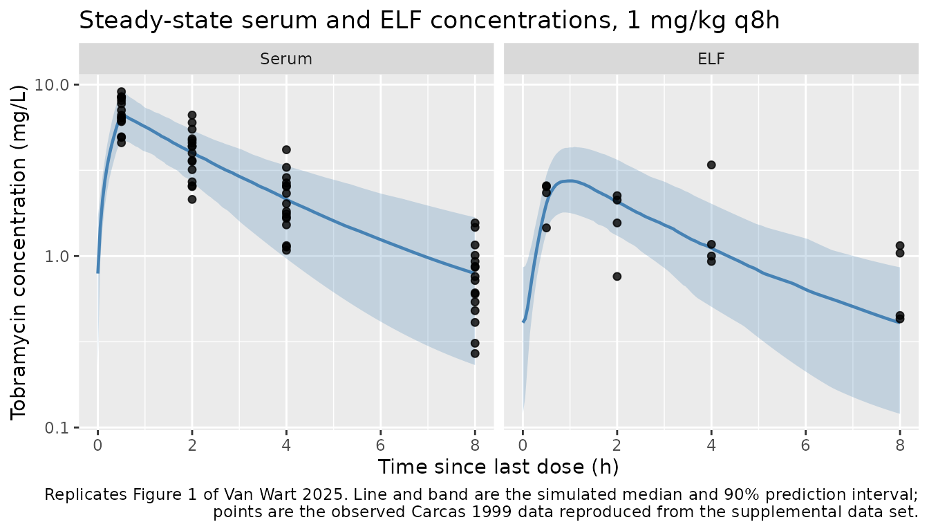
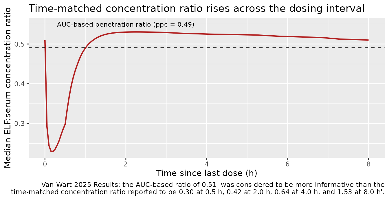
The ELF panel shows the hysteresis the paper describes: the ELF profile peaks about 30 minutes after the serum peak and its terminal decline is shallower, so the time-matched ELF:serum concentration ratio rises across the dosing interval even though the AUC-based ratio is a single number.
sim %>%
  group_by(tsld) %>%
  summarise(ratio = median(Celf / Cc), .groups = "drop") %>%
  ggplot(aes(tsld, ratio)) +
  geom_line(colour = "firebrick", linewidth = 0.8) +
  geom_hline(yintercept = ppc_tv, linetype = "dashed") +
  annotate("text", x = 0.3, y = ppc_tv * 1.12, hjust = 0,
           label = "AUC-based penetration ratio (ppc = 0.49)", size = 3) +
  labs(
    x = "Time since last dose (h)", y = "Median ELF:serum concentration ratio",
    title = "Time-matched concentration ratio rises across the dosing interval",
    caption = paste(
      "Van Wart 2025 Results: the AUC-based ratio of 0.51 'was considered to be",
      "more informative than the\ntime-matched concentration ratio reported to be",
      "0.30 at 0.5 h, 0.42 at 2.0 h, 0.64 at 4.0 h, and 1.53 at 8.0 h'."
    )
  )
Structural identity: the AUC penetration ratio is exactly
ppc
At steady state the ELF concentration returns to its starting value
over one dosing interval, so integrating the ELF ODE across the interval
gives 0 = ke0 * (ppc * AUC_serum - AUC_ELF), i.e. the
AUC-based penetration ratio equals ppc
exactly, for every subject, independent of
ke0, dose, weight, and renal function. That makes it a hard
identity rather than an approximation, and it is the tightest available
check on the ELF half of the model.
auc_by_subject <- sim %>%
  arrange(id, tsld) %>%
  group_by(id) %>%
  summarise(
    auc_serum = sum(diff(tsld) * (head(Cc, -1) + tail(Cc, -1)) / 2),
    auc_elf   = sum(diff(tsld) * (head(Celf, -1) + tail(Celf, -1)) / 2),
    ppc_i     = median(ppc),
    .groups = "drop"
  ) %>%
  mutate(ratio = auc_elf / auc_serum)

# The trapezoid on a 0.05 h grid is the only source of error here.
max_rel_err <- max(abs(auc_by_subject$ratio - auc_by_subject$ppc_i) /
                     auc_by_subject$ppc_i)
stopifnot(max_rel_err < 1e-3)
c(`max relative deviation of AUC ratio from ppc_i` = max_rel_err)
#> max relative deviation of AUC ratio from ppc_i
#>                                   2.974633e-07
Because ppc_i = ppc * exp(-etalke0) with
omega^2 = 0.0488, the penetration ratio is exactly
log-normal, and its moments are available in closed form. They match
Table 2 without any simulation at all.
omega2 <- 0.0488
analytic <- c(
  Mean   = ppc_tv * exp(omega2 / 2),
  SD     = ppc_tv * exp(omega2 / 2) * sqrt(exp(omega2) - 1),
  Median = ppc_tv
)
tibble::tibble(
  Statistic = names(analytic),
  `Closed form` = as.numeric(analytic),
  `Simulated (n = 200)` = c(mean(auc_by_subject$ratio),
                            sd(auc_by_subject$ratio),
                            median(auc_by_subject$ratio)),
  `Van Wart 2025 Table 2` = c(0.51, 0.12, 0.49)
) %>%
  knitr::kable(digits = 3,
caption = "ELF:serum AUC0-8 penetration ratio: closed form, simulation, and published values.")| Statistic | Closed form | Simulated (n = 200) | Van Wart 2025 Table 2 |
|---|---|---|---|
| Mean | 0.503 | 0.498 | 0.51 |
| SD | 0.112 | 0.113 | 0.12 |
| Median | 0.491 | 0.484 | 0.49 |
PKNCA validation
NCA is computed over the final steady-state dosing interval, with
time re-zeroed at the last dose so that Tmax is directly comparable to
Table 2. Serum and ELF are stacked into one concentration frame with a
matrix grouping variable, which keeps both outputs in a
single comparison table.
nca_conc <- sim %>%
  select(id, tsld, Serum = Cc, ELF = Celf) %>%
  tidyr::pivot_longer(c(Serum, ELF), names_to = "matrix", values_to = "Cc") %>%
  filter(!is.na(Cc)) %>%
  rename(time = tsld)

# Guarantee a time-zero record per (matrix, id); the simulation grid already
# starts at the dose time, so this only de-duplicates.
nca_conc <- nca_conc %>%
  distinct(matrix, id, time, .keep_all = TRUE) %>%
  arrange(matrix, id, time)
stopifnot(all(nca_conc %>% count(matrix, id) %>% pull(n) == length(seq(0, tau, by = 0.05))))

nca_dose <- cohort %>%
  select(id, amt = amt_mg) %>%
  tidyr::crossing(matrix = c("Serum", "ELF")) %>%
  mutate(time = 0)

conc_obj <- PKNCA::PKNCAconc(nca_conc, Cc ~ time | matrix + id,
                             concu = "mg/L", timeu = "h")
dose_obj <- PKNCA::PKNCAdose(nca_dose, amt ~ time | matrix + id, doseu = "mg")

intervals <- data.frame(
  start = 0, end = tau,
  cmax = TRUE, tmax = TRUE, cmin = TRUE, auclast = TRUE, cav = TRUE
)

nca_res <- PKNCA::pk.nca(
  PKNCA::PKNCAdata(conc_obj, dose_obj, intervals = intervals)
)
Comparison against published NCA
Table 2 of Van Wart 2025 reports mean, SD, median, and range for the
simulated steady-state metrics. ncaComparisonTable()
aggregates the simulated per-subject values with the median, so the
published medians are used as the reference.
published <- tibble::tribble(
  ~matrix, ~PPTESTCD,  ~PPORRES,
  "Serum", "cmax",         6.56,
  "Serum", "auclast",     20.0,
  "ELF",   "cmax",         2.70,
  "ELF",   "tmax",         1.0,
  "ELF",   "auclast",      9.75
)

cmp <- nlmixr2lib::ncaComparisonTable(
  simulated = nca_res,
  reference = published,
  by        = "matrix",
  units     = c(cmax = "mg/L", auclast = "mg*h/L", tmax = "h"),
  tolerance_pct = 20
)

knitr::kable(
  cmp,
  caption = paste(
    "Simulated (n = 200) vs. published (n = 1,000) steady-state NCA,",
    "Van Wart 2025 Table 2 medians. * differs from reference by > 20%."
  ),
  align = c("l", "l", "r", "r", "r")
)| NCA parameter | matrix | Reference | Simulated | % diff |
|---|---|---|---|---|
| Cmax (mg/L) | Serum | 6.56 | 6.78 | +3.4% |
| Cmax (mg/L) | ELF | 2.7 | 2.76 | +2.1% |
| Tmax (h) | ELF | 1 | 0.95 | -5.0% |
| AUClast (mg*h/L) | Serum | 20 | 21.1 | +5.6% |
| AUClast (mg*h/L) | ELF | 9.75 | 10.1 | +3.4% |
attr(cmp, "footnote")
#> NULL
Table 2 also reports dispersion, which the comparison table above does not carry. The full side-by-side is worth showing because one row does not agree.
sim_stats <- nca_res$result %>%
  filter(PPTESTCD %in% c("cmax", "tmax", "auclast")) %>%
  group_by(matrix, PPTESTCD) %>%
  summarise(Mean = mean(PPORRES), SD = sd(PPORRES),
            Median = median(PPORRES), .groups = "drop")

published_stats <- tibble::tribble(
  ~matrix, ~PPTESTCD,  ~`Mean (paper)`, ~`SD (paper)`, ~`Median (paper)`,
  "Serum", "cmax",       6.60,  0.76,  6.56,
  "ELF",   "cmax",       2.79,  0.65,  2.70,
  "ELF",   "tmax",       1.0,   0.1,   1.0,
  "Serum", "auclast",   20.5,   5.2,  20.0,
  "ELF",   "auclast",   10.3,   3.5,   9.75
)

published_stats %>%
  left_join(sim_stats, by = c("matrix", "PPTESTCD")) %>%
  mutate(Metric = nlmixr2lib::ncaParamLabel(PPTESTCD)) %>%
  select(Matrix = matrix, Metric,
         `Mean (paper)`, `Mean (sim)` = Mean,
         `SD (paper)`, `SD (sim)` = SD,
         `Median (paper)`, `Median (sim)` = Median) %>%
  knitr::kable(digits = 2,
caption = "Steady-state NCA dispersion: Van Wart 2025 Table 2 vs. this simulation.")| Matrix | Metric | Mean (paper) | Mean (sim) | SD (paper) | SD (sim) | Median (paper) | Median (sim) |
|---|---|---|---|---|---|---|---|
| Serum | Cmax | 6.60 | 6.89 | 0.76 | 1.32 | 6.56 | 6.78 |
| ELF | Cmax | 2.79 | 2.89 | 0.65 | 0.77 | 2.70 | 2.76 |
| ELF | Tmax | 1.00 | 0.97 | 0.10 | 0.10 | 1.00 | 0.95 |
| Serum | AUClast | 20.50 | 21.35 | 5.20 | 5.17 | 20.00 | 21.13 |
| ELF | AUClast | 10.30 | 10.63 | 3.50 | 3.56 | 9.75 | 10.08 |
Every central-tendency value agrees closely, and so does every dispersion except one. The serum and ELF AUC0-8 SDs in particular land almost exactly on the published values (5.17 vs. 5.20 and 3.56 vs. 3.50). The single discrepancy is the dispersion of serum Cmax: the paper reports SD 0.76 on a mean of 6.60 (11.5% CV) whereas simulating from the published OMEGA gives SD 1.32 on a mean of 6.89 (19% CV). See the Errata below.
Assumptions and deviations
- Cohort size. The paper simulated 1,000 bootstrapped patients; this vignette simulates 200 (the nlmixr2lib per-arm cap). Means, SDs, and medians are stable at that size, but the minimum and maximum in Table 2 are extreme order statistics of an n = 1,000 sample and are therefore not compared.
- Bootstrapping. Covariates are resampled with replacement from the 16 published analysis subjects, as the paper describes (“after bootstrapping from the population of model development patients”). New random effects are drawn from the published OMEGA for each simulated subject.
- Dose. 1 mg/kg, exactly as Table 2 specifies. The underlying clinical study adjusted doses to hit target peak and trough concentrations, and the published analysis data set reflects those adjusted doses; the simulation does not reproduce that adjustment because Table 2 does not.
- Race and ethnicity are not reported by Van Wart 2025 or Carcas 1999 and are not used by the model.
- The residual error is not applied to the profile figures or to the
NCA;
CcandCelfare individual predictions. Thesimcolumn returned byrxSolve()carries the residual error if it is needed.
Errata and as-published quirks
-
The creatinine clearance formula is asymmetric between the sexes. The supplemental
$PKblock computes, verbatim:BSA=0.0235*(WTKG**0.51456)*(HTCM**0.42246) ; Gehan and George IF(SEXF.EQ.0) THEN CLCR = (140.0-AGE)*WTKG/(72.0*SCR)*(1.73/BSA) ; Males, in mL/min/1.73 m^2 ELSE CLCR = ((140.0-AGE)*WTKG/(72.0*SCR))*0.85 ; Females, mL/min/1.73 m^2 ENDIFThe male branch normalises to 1.73 m^2 but applies no sex factor; the female branch applies the conventional 0.85 sex factor but is not BSA-normalised, even though its comment claims the same units. A conventional implementation would apply both to both sexes. The model file reproduces the code as published, because the reported fixed effects – in particular
lclande_crcl_cl– were estimated conditional on exactly these values. Users who want a conventional CRCL should recomputelclaccordingly rather than editing the derivation in place. Serum Cmax variability is lower in Table 2 than the published OMEGA implies. Simulating from
omega^2(Vc) = 0.0488(22.4% CV) plus the 50-84 kg weight spread gives a serum Cmax CV near 19% (SD 1.32 / mean 6.89), but Table 2 reports 11.5% (SD 0.76 / mean 6.60), with a range of 4.78-9.64 mg/L. Serum AUC0-8 dispersion matches almost exactly (SD 5.17 simulated vs. 5.20 published) and both ELF metrics agree well, so this is specific to Cmax, the metric most sensitive toVc. The most likely explanation is that the paper’s bootstrap resampled each development subject’s empirical Bayes parameters rather than drawing fresh etas: with only four serum samples per patient, all inside one dosing interval,Vcis weakly informed and its EBEs would be heavily shrunk toward the typical value. The paper does not state which was done, so this is not resolvable from the source. The model file encodes Table 1’s OMEGA as published; no value was tuned to close the gap.Vphas noini()entry. Table 1 footnote b states that “Vc and Vp were constrained to have the same value during model fitting”, and the control stream implements it asVP = TVVC– the typical central volume, withoutETA(2). The model derivesvp <- exp(lvc)so the constraint cannot be broken by re-estimatinglvc, and so thatvpcorrectly carries no IIV. The resulting Vss of 20.8 L (0.297 L/kg at 70 kg) is what the footnote reports.The three IIV variances are constrained equal. Table 1 footnote c states that the magnitude of IIV for CL, Vc, and k30 “was constrained to have the same estimated value during model fitting”, implemented as one
$OMEGA BLOCK(1)followed by twoSAMEblocks – one shared variance, three independent etas, no covariances. nlmixr2 has no cross-omega equality constraint, so the value 0.0488 is written three times; re-estimating this model would free them.Subject 6 has no 0.5 h serum sample. The Results text states that “tobramycin concentrations in serum were measured for all patients at each of the four time points”, but the supplemental analysis data set contains 63 serum records, not 64: subject 6 has serum values only at 2, 4, and 8 h. The data set is authoritative here.
The ELF compartment does not conserve mass with the central compartment.
DADT(1)contains no-K13*A(1)term, so drug appearing in ELF is not removed from serum. This is deliberate and is stated in the paper (“without impacting the serum PK data fitting”): the ELF compartment is a partitioned effect compartment used to read out a site-of-action exposure, not a physiologic distribution compartment. Do not interpretke0andppcas transfer clearances.