Osimertinib exposure-response for ILD and LVEF events (Johnson 2024)
Source:vignettes/articles/Johnson_2024_osimertinib_exposure_response.Rmd
Johnson_2024_osimertinib_exposure_response.RmdSource and models
- Citation: Johnson M, Lin YW, Schmidt H, Sunnaker M, Van Maanen E, Huang X, Rukazenkov Y, Tomkinson H, Vishwanathan K. Exposure-response modelling of osimertinib in patients with non-small cell lung cancer. Br J Clin Pharmacol. 2024;90(12):3263-3276. doi:10.1111/bcp.16199
- Article: https://doi.org/10.1111/bcp.16199
- PMC open-access copy: https://pmc.ncbi.nlm.nih.gov/articles/PMC11602960/
- Supplementary Appendix (logistic-regression model form, Tables S1-S11) published with the open-access article. A correction notice of 30 August 2024 updated reference 12 only and changes no model value.
Johnson 2024 relates the steady-state exposure (AUCss) of osimertinib, and of its active metabolite AZ5104, to efficacy and safety endpoints across the first-line, second-or-later-line and adjuvant osimertinib programme. The safety endpoints with a fitted model are interstitial lung disease (ILD) and left ventricular ejection fraction (LVEF) decrease events, each modelled by a penalized (Firth) logistic regression. Osimertinib and AZ5104 exposures are highly correlated (Figure S1), so each endpoint was fitted twice – once on each exposure – and never with both. That gives four independent models:
| Model | Endpoint | Exposure | Covariates | Source |
|---|---|---|---|---|
Johnson_2024_osimertinib_ild_osimertinib |
prob_ild |
log(AUC_OSIMERTINIB) |
RACE_JAPANESE, RACE_ASIAN
|
Table 1, Model 3 |
Johnson_2024_osimertinib_ild_az5104 |
prob_ild |
log(AUC_AZ5104) |
RACE_JAPANESE, RACE_ASIAN
|
Table S7, Model 3 |
Johnson_2024_osimertinib_lvef_osimertinib |
prob_lvef_decrease |
log(AUC_OSIMERTINIB) |
LVEF_BL |
Table 2, final model |
Johnson_2024_osimertinib_lvef_az5104 |
prob_lvef_decrease |
log(AUC_AZ5104) |
LVEF_BL |
Table 2, final model |
The models carry no PK layer: exposure is an input column. Johnson
2024 derived it as AUCss = dose / (CL/F)_i from the individual apparent
clearances of the programme’s population PK model, published as Johnson
2025 and packaged as Johnson_2025_osimertinib. This
vignette uses that model to build the exposure of a virtual cohort.
mod_ild_osi  <- readModelDb("Johnson_2024_osimertinib_ild_osimertinib")
mod_ild_az   <- readModelDb("Johnson_2024_osimertinib_ild_az5104")
mod_lvef_osi <- readModelDb("Johnson_2024_osimertinib_lvef_osimertinib")
mod_lvef_az  <- readModelDb("Johnson_2024_osimertinib_lvef_az5104")
mod_pk       <- readModelDb("Johnson_2025_osimertinib")

mw_osimertinib <- 499.62 # g/mol, C28H33N7O2 (as in Johnson_2025_osimertinib)
fm_az5104      <- 0.25   # fixed parent-to-AZ5104 fraction of the PK model
What is not packaged, and why:
- Efficacy (PFS / DFS). Johnson 2024 analysed efficacy with Kaplan-Meier curves by AUCss quartile and Cox proportional-hazards regressions (Figure 1, Table S5). A Cox model leaves the baseline hazard unestimated, so it cannot be simulated, and the paper concludes there is no exposure-efficacy relationship in any line of therapy. The Burr baseline hazard mentioned in the Figure S3 caption is not reported.
-
Rash and diarrhoea. Analysed descriptively only
(Figure 4); the exposure-response model for these endpoints is the
earlier
Brown_2017_osimertinibanalysis (reference 18).
Population
The ILD and LVEF models were fitted to osimertinib-treated patients in the first-line (AURA, FLAURA; N = 338) and second-or-later-line (AURA, AURA extension, AURA2, AURA3; N = 1026) settings with a computable AUCss (Johnson 2024 Methods, Table S1). Across these 1364 patients (Table S3) the median age was about 62 years (range 25-91), the median weight 60-62 kg (29-122 kg), 65% were female, and 62% were Asian: by grouped race 18.6% Japanese, 20.3% Chinese, 23.7% other Asian, 27.5% White and 9.9% other. Doses were 20-240 mg once daily in AURA and 80 mg once daily elsewhere. The safety analyses used the FIRST dose a patient received to compute AUCss. Comparator EGFR-TKI, chemotherapy and placebo patients appear in the paper’s figures for comparison only and were not part of any fit. The adjuvant ADAURA study (N = 325) was used to check the ILD and LVEF predictions externally.
The LVEF analysis covered 936 patients: 4 at 40 mg, 909 at 80 mg, 21 at 160 mg and 2 at 240 mg, with 0, 35, 1 and 0 events (Results). The ILD analysis had 51 events across the AUCss quartiles of Figure 2A.
Source trace
| Element | Value | Source location |
|---|---|---|
Logistic model form
log(p/(1-p)) = alpha + beta_0 * C_i + covariate terms
|
– | Supplementary Methods, ‘Logistic regression for ILD/LVEF’ |
Exposure C_i = natural log of AUCss in nM*h |
– | Results (‘log-transformed … AUCss’); Figures 2 and 3 axes; checked below |
| ILD, osimertinib: intercept / exposure / Japanese / Asian non-Japanese | -9.35 / 0.628 / 1.14 / -0.567 | Table 1, Model 3 |
| ILD, AZ5104: intercept / exposure / Japanese / Asian non-Japanese | -7.46 / 0.559 / 1.17 / -0.551 | Table S7, Model 3 |
| LVEF, osimertinib: intercept / slope / baseline LVEF | -6.36 / 0.921 / -0.087 | Table 2 (and Table S10) |
| LVEF, AZ5104: intercept / slope / baseline LVEF | -4.38 / 0.927 / -0.087 | Table 2 (and Table S11) |
| AUCss = dose / (CL/F)_i, first dose received | – | Methods, ‘Estimation of plasma exposure’ |
| Population PK model for CL/F | Johnson_2025_osimertinib |
Reference 23; NONMEM code in the Supplementary Methods |
| Placebo extrapolation 0.009% (osimertinib) and 0.06% (AZ5104) | – | Results, ‘Model simulations’ |
| Event counts by dose for LVEF | 0/4, 35/909, 1/21, 0/2 | Results, ‘Model-based exposure and LVEF analysis’ |
Placeholder residual addSd_prob_*
|
0.001, fixed | Not from source (Bernoulli likelihood) |
Check 1 – the exposure enters as a natural log of AUCss in nM*h
Johnson 2024 states that the LVEF models used “log-transformed” AUCss but does not say so for ILD, and neither table gives the exposure unit. The ILD model settles both: evaluated on the natural log of AUCss in nMh, the Table 1 Model 3 estimates reproduce the three predicted-mean curves of Figure 2C at the quartile boundaries printed on its axis. On a linear scale, or with AUCss in ngh/mL or ug*h/mL, the curves would be several-fold off.
solve_er <- function(model, output, data) {
  ev <- data |> dplyr::mutate(id = dplyr::row_number(), time = 0, amt = 0, evid = 0L)
  as.data.frame(rxode2::rxSolve(model, events = ev, returnType = "data.frame"))[[output]]
}

auc_axis <- c(6584.57, 9689.56, 12910.9, 21683.3) # Figure 2C x-axis ticks, nM*h

# Predicted-mean lines read off Figure 2C at the first and last tick.
fig2c <- tibble::tribble(
  ~race_group,            ~AUC_OSIMERTINIB, ~published,
  "Non-Asian",            6584.57,          0.021,
  "Non-Asian",            21683.3,          0.045,
  "Japanese",             6584.57,          0.065,
  "Japanese",             21683.3,          0.127,
  "Asian (non-Japanese)", 6584.57,          0.012,
  "Asian (non-Japanese)", 21683.3,          0.025
) |>
  dplyr::mutate(
    RACE_JAPANESE = as.integer(race_group == "Japanese"),
    RACE_ASIAN    = as.integer(race_group == "Asian (non-Japanese)")
  )
fig2c$packaged <- solve_er(mod_ild_osi, "prob_ild", fig2c)
#> Warning: multi-subject simulation without without 'omega'

fig2c |>
  dplyr::select(race_group, AUC_OSIMERTINIB, published, packaged) |>
  dplyr::mutate(packaged = round(packaged, 4)) |>
  dplyr::rename(
    "Race group" = race_group, "AUCss (nM*h)" = AUC_OSIMERTINIB,
    "Figure 2C (read off)" = published, "Packaged model" = packaged
  ) |>
knitr::kable()| Race group | AUCss (nM*h) | Figure 2C (read off) | Packaged model |
|---|---|---|---|
| Non-Asian | 6584.57 | 0.021 | 0.0213 |
| Non-Asian | 21683.30 | 0.045 | 0.0439 |
| Japanese | 6584.57 | 0.065 | 0.0637 |
| Japanese | 21683.30 | 0.127 | 0.1257 |
| Asian (non-Japanese) | 6584.57 | 0.012 | 0.0122 |
| Asian (non-Japanese) | 21683.30 | 0.025 | 0.0254 |
stopifnot(
  # The figure is read to about +/- 0.003; a wrong scale or unit misses by
  # far more than that.
  all(abs(fig2c$packaged - fig2c$published) < 0.006)
)
grid_2c <- tidyr::expand_grid(
  AUC_OSIMERTINIB = exp(seq(log(5000), log(30000), length.out = 60)),
  race_group = c("Non-Asian", "Japanese", "Asian (non-Japanese)")
) |>
  dplyr::mutate(
    RACE_JAPANESE = as.integer(race_group == "Japanese"),
    RACE_ASIAN    = as.integer(race_group == "Asian (non-Japanese)")
  )
grid_2c$p <- solve_er(mod_ild_osi, "prob_ild", grid_2c)
#> Warning: multi-subject simulation without without 'omega'

ggplot(grid_2c, aes(AUC_OSIMERTINIB, p, linetype = race_group)) +
  geom_line(linewidth = 0.8) +
  geom_vline(xintercept = auc_axis, linetype = "dotted", colour = "grey50") +
  scale_y_continuous(labels = scales::percent) +
  labs(x = "Osimertinib AUCss (nM*h)", y = "Probability of an ILD event",
       linetype = NULL) +
  theme_bw() +
  theme(legend.position = "bottom")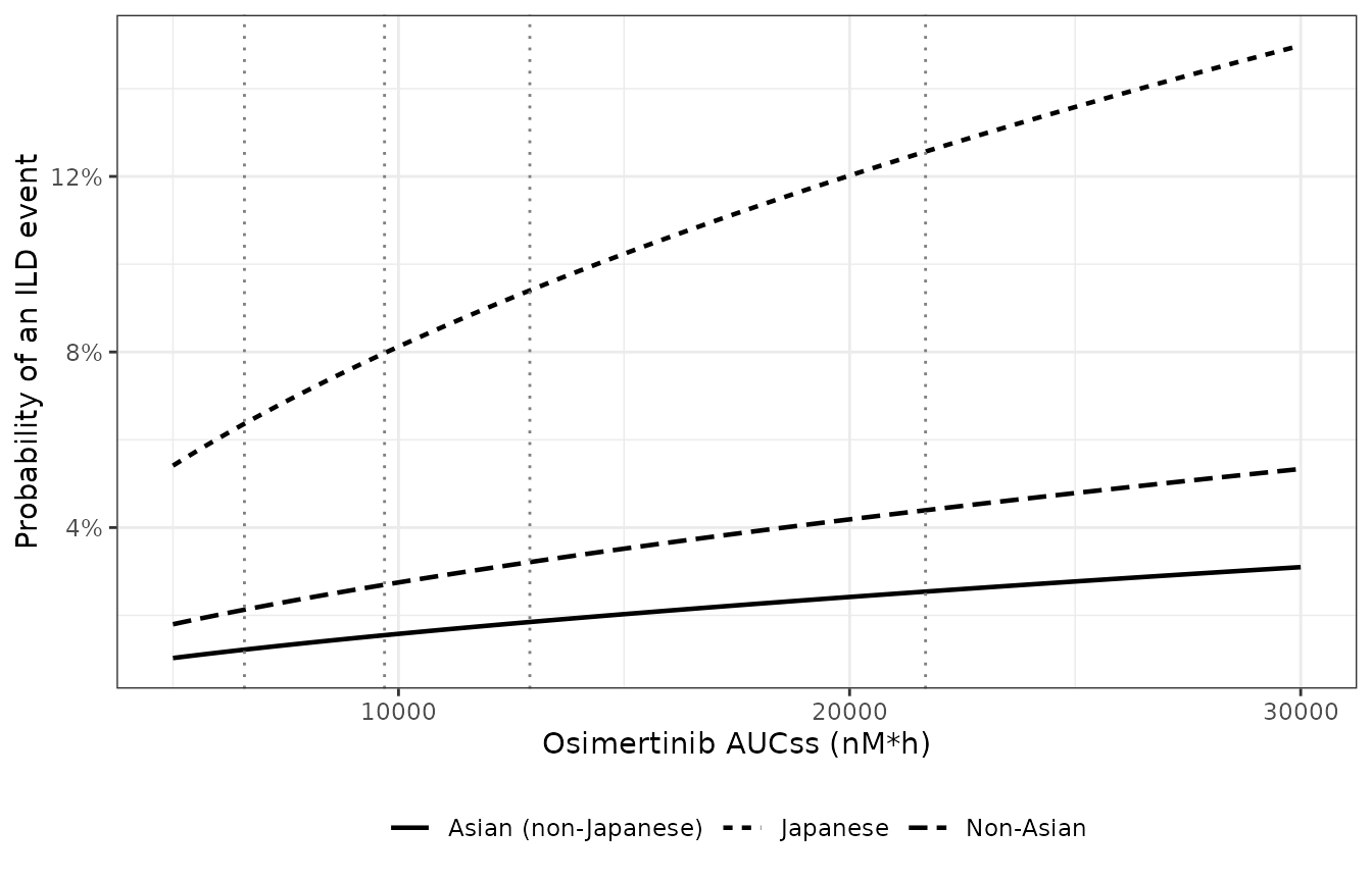
Replicates Figure 2C of Johnson 2024: predicted ILD probability against osimertinib AUCss by race group (final model). Dashed lines mark the quartile boundaries printed on the published axis.
Check 2 – the published placebo extrapolation
Johnson 2024 quotes the ILD probability of a placebo patient (“AUCss
= 0”) as 0.009% from the osimertinib model and 0.06% from the AZ5104
model, “calculated from the intercept estimates in Table 1 and Table
S7”. Because the exposure enters as log(AUCss), a literal
zero exposure gives a probability of exactly 0; the quoted values are
the probabilities at log(AUCss) = 0, i.e.
expit(intercept) for a non-Asian patient. The packaged
intercepts reproduce both numbers.
p_int <- c(
  osimertinib = solve_er(mod_ild_osi, "prob_ild",
                         data.frame(AUC_OSIMERTINIB = 1, RACE_JAPANESE = 0, RACE_ASIAN = 0)),
  az5104      = solve_er(mod_ild_az, "prob_ild",
                         data.frame(AUC_AZ5104 = 1, RACE_JAPANESE = 0, RACE_ASIAN = 0))
)
round(100 * p_int, 4)
#> osimertinib      az5104
#>      0.0087      0.0575

stopifnot(
  round(100 * p_int[["osimertinib"]], 3) == 0.009,
  round(100 * p_int[["az5104"]], 2) == 0.06
)
Virtual cohort
The cohort has 200 virtual patients in each of the three race groups
of the ILD model (non-Asian, Japanese, Asian non-Japanese). Each patient
is evaluated at 40, 80 and 160 mg once daily – the doses of Figures 2D
and 3B – so the dose comparisons are paired. Body weight and baseline
albumin follow the truncated log-normal distributions used in the
Johnson_2025_osimertinib vignette (medians 61 kg and 39
g/L). Within the non-Asian group the White to other split, and within
the Asian non-Japanese group the Chinese to other-Asian split, follow
Table S3 (first-line plus second-or-later-line columns); the PK model
needs these finer groups for the AZ5104 clearance. Baseline LVEF is not
reported by Johnson 2024; it is drawn from a normal distribution with
mean 63% and SD 6%, restricted to 50-80% (an assumption, see below).
The between-patient random effects of the PK model are drawn in base
R and passed to rxSolve() as parameters, so the cohort does
not depend on the random-number stream of the installed rxode2.
set.seed(20241101)
n_per_group <- 200
race_groups <- c("Non-Asian", "Japanese", "Asian (non-Japanese)")

sample_truncated_lognorm <- function(n, lo, hi, median_val, sd_log) {
  out <- numeric(0)
  while (length(out) < n) {
    draw <- exp(rnorm(n, mean = log(median_val), sd = sd_log))
    out <- c(out, draw[draw >= lo & draw <= hi])
  }
  out[seq_len(n)]
}

group <- rep(race_groups, each = n_per_group)
n_sub <- length(group)
u <- runif(n_sub)
# Table S3 (first-line + second-or-later-line): White 375 vs other non-Asian
# 135; Chinese 277 vs Asian non-Chinese non-Japanese 323.
pk_race <- dplyr::case_when(
  group == "Non-Asian" & u < 375 / 510 ~ "White",
  group == "Non-Asian" ~ "Other",
  group == "Japanese" ~ "Japanese",
  u < 277 / 600 ~ "Chinese",
  TRUE ~ "Asian_oth"
)

cohort <- tibble::tibble(
  id = seq_len(n_sub),
  race_group = group,
  WT  = sample_truncated_lognorm(n_sub, lo = 29, hi = 122, median_val = 61, sd_log = 0.21),
  ALB = sample_truncated_lognorm(n_sub, lo = 17, hi = 53.3, median_val = 39, sd_log = 0.13),
  RACE_CHINESE   = as.integer(pk_race == "Chinese"),
  RACE_JAPANESE  = as.integer(pk_race == "Japanese"),
  RACE_ASIAN_OTH = as.integer(pk_race == "Asian_oth"),
  RACE_OTHER     = as.integer(pk_race == "Other"),
  LVEF_BL = pmin(pmax(rnorm(n_sub, mean = 63, sd = 6), 50), 80)
)

omega <- rxode2::rxode2(mod_pk)$omega
#> ℹ parameter labels from comments will be replaced by 'label()'
eta <- matrix(rnorm(n_sub * nrow(omega)), n_sub) %*% chol(omega)
colnames(eta) <- rownames(omega)

# One observation record per patient is enough: the individual apparent
# clearances are time-invariant.
pk_events <- cohort |>
  dplyr::transmute(id, time = 0, amt = 0, evid = 0L, dvid = 1L,
                   WT, ALB, RACE_CHINESE, RACE_JAPANESE, RACE_ASIAN_OTH, RACE_OTHER)
pk_par <- rxode2::rxSolve(rxode2::zeroRe(mod_pk), events = pk_events,
                          params = data.frame(id = cohort$id, eta),
                          returnType = "data.frame")
#> ℹ parameter labels from comments will be replaced by 'label()'
#> Warning: multi-subject simulation without without 'omega'
cohort <- cohort |>
  dplyr::mutate(cl = pk_par$cl, cl_az5104 = pk_par$cl_az5104)

exposure <- tidyr::expand_grid(cohort, dose = c(40, 80, 160)) |>
  dplyr::mutate(
    AUC_OSIMERTINIB = dose / cl * 1e6 / mw_osimertinib,
    AUC_AZ5104      = fm_az5104 * dose / cl_az5104 * 1e6 / mw_osimertinib,
    RACE_JAPANESE   = as.integer(race_group == "Japanese"),
    RACE_ASIAN      = as.integer(race_group == "Asian (non-Japanese)")
  )
The simulated osimertinib AUCss by dose sits where the box plots of Figure 2A put it (medians near 5500, 11 000 and 22 000 nM*h), and the random effects carry the CL/F variability of the PK model (44.9% CV).
exposure |>
  dplyr::group_by(dose) |>
  dplyr::summarise(
    `Median osimertinib AUCss (nM*h)` = round(median(AUC_OSIMERTINIB)),
    `5th percentile` = round(quantile(AUC_OSIMERTINIB, 0.05)),
    `95th percentile` = round(quantile(AUC_OSIMERTINIB, 0.95)),
    `Median AZ5104 AUCss (nM*h)` = round(median(AUC_AZ5104)),
    .groups = "drop"
  ) |>
  dplyr::rename("Dose (mg QD)" = dose) |>
knitr::kable()| Dose (mg QD) | Median osimertinib AUCss (nM*h) | 5th percentile | 95th percentile | Median AZ5104 AUCss (nM*h) |
|---|---|---|---|---|
| 40 | 5493 | 2824 | 11581 | 570 |
| 80 | 10986 | 5647 | 23162 | 1140 |
| 160 | 21973 | 11294 | 46323 | 2280 |
typical_auc_80 <- 80 / exp(rxode2::rxode2(mod_pk)$theta[["lcl"]]) * 1e6 / mw_osimertinib
#> ℹ parameter labels from comments will be replaced by 'label()'
sd_log_cl <- sd(log(cohort$cl))
c(typical_auc_80 = typical_auc_80, sd_log_cl = sd_log_cl)
#> typical_auc_80      sd_log_cl
#>   1.119732e+04   4.371252e-01

stopifnot(
  # The cohort median is near the typical-patient value; covariates move it
  # by a few percent only.
  abs(median(exposure$AUC_OSIMERTINIB[exposure$dose == 80]) / typical_auc_80 - 1) < 0.1,
  # The random effects were applied (omega of CL/F = 0.43 on the log scale);
  # covariates add a little on top.
  sd_log_cl > 0.35, sd_log_cl < 0.6
)
Replicate Figure 2D – ILD probability by dose and race
Johnson 2024 Figure 2D shows the predicted mean ILD probability at 40, 80 and 160 mg in each race group and in the overall population. The overall value here weights the three groups by their share of the first-line plus second-or-later-line population of Table S3 (non-Asian 510, Japanese 254, Asian non-Japanese 600 of 1364).
exposure$p_ild_osi <- solve_er(mod_ild_osi, "prob_ild", exposure)
#> Warning: multi-subject simulation without without 'omega'
exposure$p_ild_az  <- solve_er(mod_ild_az, "prob_ild", exposure)
#> Warning: multi-subject simulation without without 'omega'

group_weight <- c("Non-Asian" = 510, "Japanese" = 254, "Asian (non-Japanese)" = 600) / 1364

by_group <- exposure |>
  dplyr::group_by(race_group, dose) |>
  dplyr::summarise(p_osi = mean(p_ild_osi), p_az = mean(p_ild_az), .groups = "drop")
overall <- by_group |>
  dplyr::mutate(w = group_weight[race_group]) |>
  dplyr::group_by(dose) |>
  dplyr::summarise(p_osi = sum(w * p_osi), p_az = sum(w * p_az), .groups = "drop") |>
  dplyr::mutate(race_group = "Overall population")

# Grey predicted means read off Figure 2D.
fig2d <- tibble::tribble(
  ~race_group,            ~dose, ~published,
  "Non-Asian",            40,    0.020,
  "Non-Asian",            80,    0.032,
  "Non-Asian",            160,   0.047,
  "Japanese",             40,    0.067,
  "Japanese",             80,    0.095,
  "Japanese",             160,   0.142,
  "Asian (non-Japanese)", 40,    0.012,
  "Asian (non-Japanese)", 80,    0.020,
  "Asian (non-Japanese)", 160,   0.028,
  "Overall population",   40,    0.025,
  "Overall population",   80,    0.038,
  "Overall population",   160,   0.057
)

cmp_2d <- dplyr::bind_rows(by_group, overall) |>
  dplyr::inner_join(fig2d, by = c("race_group", "dose"))

cmp_2d |>
  dplyr::mutate(dplyr::across(c(p_osi, p_az), ~ round(.x, 3))) |>
  dplyr::select(race_group, dose, published, p_osi, p_az) |>
  dplyr::rename(
    "Race group" = race_group, "Dose (mg QD)" = dose,
    "Figure 2D (read off)" = published,
    "Simulated, osimertinib model" = p_osi, "Simulated, AZ5104 model" = p_az
  ) |>
knitr::kable()| Race group | Dose (mg QD) | Figure 2D (read off) | Simulated, osimertinib model | Simulated, AZ5104 model |
|---|---|---|---|---|
| Asian (non-Japanese) | 40 | 0.012 | 0.012 | 0.012 |
| Asian (non-Japanese) | 80 | 0.020 | 0.018 | 0.018 |
| Asian (non-Japanese) | 160 | 0.028 | 0.027 | 0.026 |
| Japanese | 40 | 0.067 | 0.061 | 0.061 |
| Japanese | 80 | 0.095 | 0.090 | 0.087 |
| Japanese | 160 | 0.142 | 0.133 | 0.123 |
| Non-Asian | 40 | 0.020 | 0.019 | 0.021 |
| Non-Asian | 80 | 0.032 | 0.030 | 0.030 |
| Non-Asian | 160 | 0.047 | 0.045 | 0.044 |
| Overall population | 40 | 0.025 | 0.024 | 0.024 |
| Overall population | 80 | 0.038 | 0.036 | 0.035 |
| Overall population | 160 | 0.057 | 0.053 | 0.051 |
stopifnot(
  # Within 20% of the published means in every cell. The largest gap is the
  # Japanese group, which the cohort gives the overall weight distribution;
  # Johnson 2024 notes Japanese patients were lighter and had higher AUCss.
  all(abs(log(cmp_2d$p_osi / cmp_2d$published)) < log(1.2)),
  # The two exposure drivers describe the same events and agree closely.
  all(abs(log(cmp_2d$p_az / cmp_2d$p_osi)) < log(1.15))
)
cmp_2d |>
  ggplot(aes(factor(dose), p_osi)) +
  geom_col(fill = "grey75") +
  geom_point(aes(y = published), size = 2) +
  facet_wrap(~race_group, nrow = 1) +
  scale_y_continuous(labels = scales::percent) +
  labs(x = "Osimertinib dose (mg once daily)", y = "Probability of an ILD event") +
  theme_bw()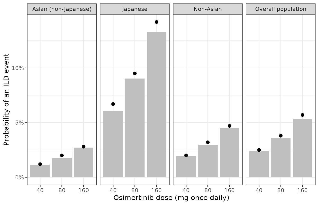
Replicates Figure 2D of Johnson 2024: predicted mean ILD probability by dose and race group (bars: simulated, osimertinib-driven model; points: values read off the published figure).
At 80 mg the observed proportions in Figure 2D (about 2.8% non-Asian, 10.4% Japanese, 2.2% Asian non-Japanese, 4.1% overall) sit on top of the predictions, as the paper reports.
Replicate Figure 3B – LVEF-decrease probability by dose
The LVEF models need a baseline LVEF, which Johnson 2024 does not
tabulate, so the absolute probabilities below depend on the assumed
baseline distribution. The dose RATIO does not: in the logistic model a
doubling of AUCss multiplies the odds by 2^slope whatever
the baseline, which gives a check that is free of that assumption.
exposure$p_lvef_osi <- solve_er(mod_lvef_osi, "prob_lvef_decrease", exposure)
#> Warning: multi-subject simulation without without 'omega'
exposure$p_lvef_az  <- solve_er(mod_lvef_az, "prob_lvef_decrease", exposure)
#> Warning: multi-subject simulation without without 'omega'

lvef_dose <- exposure |>
  dplyr::mutate(w = group_weight[race_group] / n_per_group) |>
  dplyr::group_by(dose) |>
  dplyr::summarise(p_osi = sum(w * p_lvef_osi), p_az = sum(w * p_lvef_az), .groups = "drop") |>
  dplyr::mutate(published = c(0.024, 0.043, 0.076)) # Figure 3B model predictions, read off

lvef_dose |>
  dplyr::mutate(dplyr::across(c(p_osi, p_az), ~ round(.x, 3))) |>
  dplyr::select(dose, published, p_osi, p_az) |>
  dplyr::rename(
    "Dose (mg QD)" = dose, "Figure 3B (read off)" = published,
    "Simulated, osimertinib model" = p_osi, "Simulated, AZ5104 model" = p_az
  ) |>
knitr::kable()| Dose (mg QD) | Figure 3B (read off) | Simulated, osimertinib model | Simulated, AZ5104 model |
|---|---|---|---|
| 40 | 0.024 | 0.025 | 0.024 |
| 80 | 0.043 | 0.046 | 0.044 |
| 160 | 0.076 | 0.082 | 0.080 |
# Odds ratio per doubling of dose, typical patient (exact) and published
# figure (from the read-off means).
odds <- function(p) p / (1 - p)
or_doubling <- c(
  model_exact = 2^0.921,
  figure_40_to_80 = odds(0.043) / odds(0.024),
  figure_80_to_160 = odds(0.076) / odds(0.043)
)
round(or_doubling, 2)
#>      model_exact  figure_40_to_80 figure_80_to_160
#>             1.89             1.83             1.83

stopifnot(
  # Baseline-free check: the published dose steps imply the model's
  # odds ratio per doubling of exposure.
  all(abs(log(or_doubling[-1] / or_doubling[["model_exact"]])) < log(1.15)),
  # Assumption-dependent check (baseline LVEF not reported): same order of
  # magnitude as Figure 3B at every dose.
  all(abs(log(lvef_dose$p_osi / lvef_dose$published)) < log(1.3)),
  all(diff(lvef_dose$p_osi) > 0)
)
The observed rate at 80 mg (35/909 = 3.9%) lies inside the predicted interval, while the comparator arms had 1/94 (chemotherapy) and 4/256 (comparator EGFR-TKI) events. Johnson 2024 notes that the 95% intervals at 80 mg and for the comparators largely overlap, so the exposure dependence of LVEF events is uncertain and confounded by the small number of events and the baseline LVEF.
PKNCA
Not applicable: these are static landmark exposure-response models
with no time dimension and no concentration profile. Exposure enters as
an AUCss column; the steady-state AUCs of the companion PK model are
validated with PKNCA in the Johnson_2025_osimertinib
vignette. The exposure check above confirms that the dose / CL/F
derivation used here lands on the published AUCss distribution.
Assumptions and deviations
- Exposure scale. Johnson 2024 states “log-transformed” AUCss for the LVEF models only and never gives the exposure unit. The natural log of AUCss in nM*h is used for all four models; Check 1 shows it reproduces Figure 2C, and Check 2 reproduces the quoted placebo probabilities.
-
Zero exposure. With
log(AUCss)a placebo patient (AUCss = 0) has a predicted probability of exactly 0. The paper’s quoted 0.009% / 0.06% are the probabilities atlog(AUCss) = 0. The paper itself notes that the model, fitted to osimertinib-treated patients only, underestimates the background ILD rate. -
Race encoding. The ILD models’ “Asian
(non-Japanese)” covariate is encoded as
RACE_ASIANand is mutually exclusive withRACE_JAPANESE: a Japanese patient hasRACE_ASIAN = 0. This differs from the companion PK model, whereRACE_ASIAN_OTHexcludes Chinese patients too. -
AZ5104 AUCss. Johnson 2024 does not print the
formula for the AZ5104 AUCss. It is taken as the molar steady-state
value
fm * dose / (CLm/F)_iof the PK model, with the fixed fm = 0.25. The supplementary NONMEM code scales the metabolite compartment by the AZ5104 molecular weight without a molar conversion, a 2.8% difference in AUCss that moves the logit by less than 0.02. - Placeholder residual. The source fits a Bernoulli likelihood with Firth penalization and no random effects. Each model declares its probability as the observation with a fixed additive residual of 0.001 only so that rxode2 accepts the model; it has no source counterpart.
- Virtual cohort. Body weight and albumin follow overall distributions for all race groups; Johnson 2024 notes Japanese patients were lighter, with higher AUCss, which is why the simulated Japanese means fall slightly below Figure 2D. Baseline LVEF (mean 63%, SD 6%, restricted to 50-80%) is an assumption, as the paper does not report it.
- Sensitivity refits not encoded. The LVEF refits restricted to baseline LVEF 50 to < 70% (Tables S10 and S11) and the non-final ILD Models 1, 2 and 4 (Table 1, Table S7) are not packaged.