Evolocumab popPK and LDL-C exposure-response (Kuchimanchi 2018)
Source:vignettes/articles/Kuchimanchi_2018_evolocumab.Rmd
Kuchimanchi_2018_evolocumab.Rmd
library(nlmixr2lib)
library(rxode2)
#> rxode2 5.1.2 using 2 threads (see ?getRxThreads)
#>   no cache: create with `rxCreateCache()`
library(PKNCA)
#>
#> Attaching package: 'PKNCA'
#> The following object is masked from 'package:stats':
#>
#>     filter
library(dplyr)
#>
#> Attaching package: 'dplyr'
#> The following objects are masked from 'package:stats':
#>
#>     filter, lag
#> The following objects are masked from 'package:base':
#>
#>     intersect, setdiff, setequal, union
library(tidyr)
library(ggplot2)
Evolocumab population PK and LDL-C exposure-response (Kuchimanchi 2018)
Kuchimanchi et al. (2018) characterised the population pharmacokinetics and the exposure-response relationship for evolocumab, a fully human IgG2 monoclonal antibody against proprotein convertase subtilisin/kexin type 9 (PCSK9), in patients with hypercholesterolemia. The final population PK (popPK) model (Table 3, fit to 3414 subjects pooled across 11 phase 1, 2, and 3 studies) is a one-compartment model with first-order SC absorption from a depot compartment and parallel linear plus Michaelis-Menten (target-mediated) elimination from the central compartment. Body weight entered as a power effect on CL, V, and Vmax; female sex multiplied V; statin monotherapy, ezetimibe use (functionally the statin + ezetimibe combination-therapy indicator), and baseline PCSK9 modified Vmax. The absorption rate constant (ka), SC bioavailability (F), Michaelis-Menten constant (km), and Vmax typical value were fixed in the updated phase 3 popPK model.
The companion exposure-response model (Table 4, fit to 1314 patients from 4 phase 2 studies) is an algebraic Emax relationship linking the AUC of unbound evolocumab over weeks 8 to 12 of treatment (AUCwk8-12) to the mean LDL-C reduction at weeks 10 and 12. Statin and statin + ezetimibe combination therapy lowered baseline LDL-C; heterozygous familial hypercholesterolemia (HeFH) raised it; statin co-administration also attenuated the maximum drug-induced LDL-C reduction (Emax). A regimen- effect multiplier on EC50 distinguished the once-monthly (QM) dosing arm from the once-every-2-weeks (Q2W) arm because the static Emax-on-AUC formulation cannot otherwise capture the difference in target-saturation time courses between regimens with similar AUC values.
The library packages both models as a pair, sharing this vignette:
Model file (modellib() key) |
Endpoint |
|---|---|
Kuchimanchi_2018_evolocumab |
Evolocumab serum concentration (popPK only) |
Kuchimanchi_2018_evolocumab_ldlc |
popPK + AUCwk8-12 tracker + LDL-C E-R response |
This vignette reproduces the typical-value concentration-time profiles for the two commercial regimens (140 mg SC Q2W and 420 mg SC QM), documents the parameter provenance in a source-trace table, validates the simulated NCA (PKNCA) steady-state exposures against the published mean Cmax values, and replicates the paper’s predicted maximal LDL-C reduction for the two commercial regimens at the reference patient.
Model and source
- Citation: Kuchimanchi M, Monine M, Kandadi Muralidharan K, Woodhead JL, Horner TJ. Population pharmacokinetics and exposure–response modeling and simulation for evolocumab in healthy volunteers and patients with hypercholesterolemia. J Pharmacokinet Pharmacodyn. 2019;46(2):133–148.
- Article: doi:10.1007/s10928-018-9592-y.
- No errata were identified (PubMed search
Kuchimanchi 2018 evolocumab erratum, 2026-04-24, returned no results).
Population
Kuchimanchi 2018 Table 2 (phase 1, 2, and 3 pooled column; N = 3414):
| Field | Value |
|---|---|
| N subjects | 3414 (receiving evolocumab; pooled from 5474 across all arms) |
| N observations | 16 179 evolocumab concentrations |
| N studies | 11 (1 phase 1a, 1 phase 1b, 4 phase 2, 5 phase 3) |
| Age | 18–80 years (mean 57) |
| Weight | 41–175 kg (mean 84.2) |
| Sex | 50% female / 50% male |
| Race / ethnicity | 87% White, 7% Black, 4% Asian, 2% other |
| Disease state | Healthy volunteers (phase 1a) + hypercholesterolemia patients |
| Baseline PCSK9 | Mean 402 ng/mL (range 15.5–1233) |
| Baseline albumin | Mean 4.3 g/dL (range 2.6–5.6) |
| HeFH (%) | 9% |
| Diabetes (%) | 11% |
| Statin (any) (%) | ~72% |
| Ezetimibe (%) | 12% |
| Dose range | 7–420 mg IV or SC across single- and multiple-dose regimens |
| Phase 3 regimens | 140 mg SC Q2W and 420 mg SC QM |
| Reference patient | 84 kg male, no lipid-lowering meds, baseline PCSK9 = 425 ng/mL |
The population metadata is also available programmatically via
readModelDb("Kuchimanchi_2018_evolocumab")$population.
Source trace
Every numeric value in the model file
inst/modeldb/specificDrugs/Kuchimanchi_2018_evolocumab.R is
sourced from Kuchimanchi 2018. Final estimates are the updated
phase 3 population PK model column in Table 3; Vmax
and km were fixed in that column from the phase 1+2 run
because phase 3 used only two dose regimens.
| Quantity | Source location | Value used |
|---|---|---|
| Structural model (1-cmt, linear + MM) | Methods § PopPK analysis / Figure 1a | Depot → central, CL + V·Vmax·C/(km+C) |
| F (SC bioavailability) | Table 3 | 0.72 (FIXED) |
| ka | Table 3 | 0.319 day-1 (FIXED) |
| CL | Table 3 | 0.105 L/day |
| V | Table 3 | 5.18 L |
| Vmax | Table 3 | 9.85 nM/day (FIXED) |
| km | Table 3 | 27.3 nM (FIXED) |
| Reference body weight | Methods, reference-patient definition | 84 kg (male) |
| WT exponent on CL | Table 3 | 0.276 |
| WT exponent on V | Table 3 | 1.04 |
| Female exponent on V | Table 3 | 1.11 |
| WT exponent on Vmax | Table 3 | 0.145 |
| Statin (monotherapy) exponent on Vmax | Table 3 | 1.13 |
| Statin + ezetimibe exponent on Vmax | Table 3 | 1.20 |
| Baseline PCSK9 exponent on Vmax | Table 3 | 0.194 |
| Reference PCSK9 | Methods, reference-patient definition | 425 ng/mL (= 5.9 nM) |
| IIV on CL | Table 3 | 54.3% CV |
| IIV on V | Table 3 | 28.3% CV |
| IIV on Vmax | Table 3 | 31.1% CV |
| IIV on ka | Table 3 | 74.6% CV (FIXED) |
| IIV on km | Table 3 | 0% (FIXED) |
| Full-block CL/V/Vmax omega structure | Table 3 note; Table 4 referenced but | Correlations not published — diagonal used |
| actually E-R parameters | (see Assumptions and deviations) | |
| Proportional residual error (PK) | Table 3 | 0.282 (28.2% CV) |
| Additive residual error (PK) | Table 3 | 5.41 nM (= 0.767 µg/mL at MW 141.8 kDa) |
| Evolocumab molecular weight | FDA-approved Repatha label | 141 800 g/mol |
| Typical baseline LDL-C (E-R) | Table 4 | 150 mg/dL |
| Emax (max LDL-C reduction) | Table 4 | -99.7 mg/dL |
| EC50 at Q2W (E-R) | Table 4 | 51.5 (µg/mL)·day |
Regimen multiplier reg_qm (QM/Q2W) |
Table 4 (REG) | 2.30 |
| Statin exponent on baseline LDL-C | Table 4 | 0.797 |
| Ezetimibe exponent on baseline LDL-C | Table 4 | 0.768 |
| HeFH exponent on baseline LDL-C | Table 4 | 1.28 |
| Statin exponent on Emax | Table 4 | 0.937 |
| IIV on baseline LDL-C | Table 4 | 20.0% CV |
| Additive residual error (LDL-C) | Table 4 | 19.3 mg/dL |
| Proportional residual error (LDL-C) | Table 4 | 0 (FIXED) |
| AUCwk8-12 integration window | Methods, paragraph defining E-R metric | days 56-84 (week 8 to week 12) |
PCSK9 MW (~72 kDa), used only to cross-check the paper’s nM↔︎ng/mL conversion (5.9 nM ≈ 425 ng/mL), is not a model parameter.
Virtual cohort
The original patient-level data are not public. To replicate the
paper’s reference-patient Cmax we simulate a small
typical-value cohort at the two commercial regimens (140 mg SC Q2W and
420 mg SC QM) with the model’s random effects zeroed
(rxode2::zeroRe()), i.e. a single “average” subject per
regimen matching the Methods-section reference definition (84 kg male,
no lipid-lowering medication, baseline PCSK9 = 425 ng/mL).
set.seed(20260424)

reference_covariates <- tibble::tibble(
  WT          = 84,
  SEXF        = 0L,
  CONMED_STATIN_MONO = 0L,
  CONMED_EZE         = 0L,
  PCSK9       = 425
)

make_regimen <- function(amt, ii, addl, label) {
  ev <- rxode2::et(amt = amt, cmt = "depot", ii = ii, addl = addl) |>
    rxode2::et(seq(0, 12 * 14, by = 0.5))
  df <- as.data.frame(ev)
  df$id          <- 1L
  df$WT          <- reference_covariates$WT
  df$SEXF        <- reference_covariates$SEXF
  df$CONMED_STATIN_MONO <- reference_covariates$CONMED_STATIN_MONO
  df$CONMED_EZE         <- reference_covariates$CONMED_EZE
  df$PCSK9       <- reference_covariates$PCSK9
  df$regimen     <- label
  df
}

events <- dplyr::bind_rows(
  make_regimen(amt = 140, ii = 14, addl = 11, label = "140 mg SC Q2W"),
  make_regimen(amt = 420, ii = 28, addl = 5,  label = "420 mg SC QM")  |>
    dplyr::mutate(id = 2L)
)
stopifnot(!anyDuplicated(unique(events[, c("id", "time", "evid")])))
Simulation
mod <- readModelDb("Kuchimanchi_2018_evolocumab")
ui  <- rxode2::rxode(mod)
#> ℹ parameter labels from comments will be replaced by 'label()'

# Typical-value prediction: no between-subject variability and no residual error.
mod_typical <- rxode2::zeroRe(ui)
sim <- rxode2::rxSolve(mod_typical, events = events, keep = c("regimen"))
#> ℹ omega/sigma items treated as zero: 'etalcl', 'etalvc', 'etalvmax', 'etalka'
#> Warning: multi-subject simulation without without 'omega'
Replicate published figures
ggplot(sim, aes(time, Cc, colour = regimen)) +
  geom_line(linewidth = 0.7) +
  labs(x = "Time (day)", y = "Serum evolocumab (µg/mL)",
       colour = "Regimen",
       title = "Typical serum evolocumab concentration-time profiles",
       caption = "Reference patient: 84 kg male, no lipid-lowering Rx, PCSK9 = 425 ng/mL.") +
  theme_minimal(base_size = 11)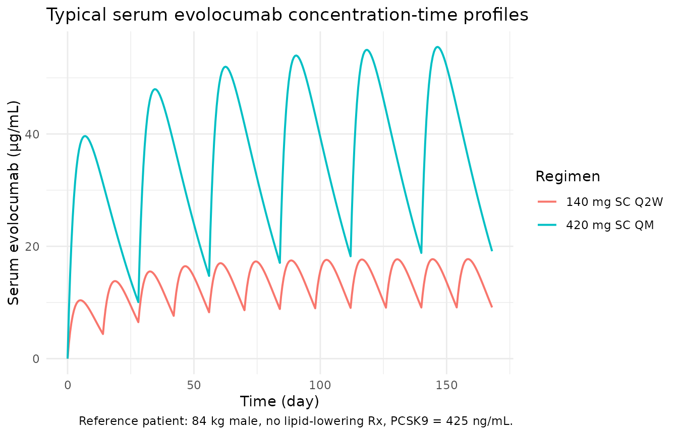
Typical serum evolocumab concentration time-course after 140 mg SC Q2W and 420 mg SC QM (reference patient). Replicates the shape and range of Figure 4a/4c of Kuchimanchi 2018.
ggplot(sim, aes(time, Cc, colour = regimen)) +
  geom_line(linewidth = 0.7) +
  scale_y_log10() +
  labs(x = "Time (day)", y = "Serum evolocumab (µg/mL, log)",
       colour = "Regimen") +
  theme_minimal(base_size = 11)
#> Warning in scale_y_log10(): log-10 transformation introduced infinite values.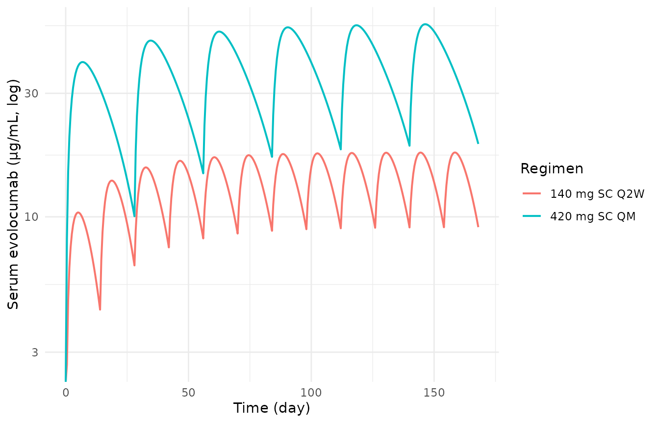
Same simulation on a log scale, showing the dose-proportional scaling between Q2W and QM trough concentrations.
PKNCA validation
Use PKNCA to compute steady-state AUC, Cmax, Tmax, Cmin, and Cavg over the last dosing interval of each regimen (days 154–168 for Q2W, days 140–168 for QM). We keep observations between the final dose and the end of simulation, one per regimen, so NCA runs on the steady-state window.
tau_by_regimen <- c("140 mg SC Q2W" = 14, "420 mg SC QM" = 28)

sim_nca <- sim |>
  dplyr::filter(!is.na(Cc)) |>
  dplyr::mutate(
    tau       = tau_by_regimen[regimen],
    dose_last = 12 * 14 - tau
  ) |>
  dplyr::filter(time >= dose_last) |>
  dplyr::mutate(tad = time - dose_last) |>
  dplyr::select(id, time, tad, Cc, regimen)

dose_df <- events |>
  dplyr::filter(evid == 1) |>
  dplyr::group_by(id, regimen) |>
  dplyr::slice_tail(n = 1) |>     # final dose only
  dplyr::ungroup() |>
  dplyr::select(id, time, amt, regimen)

conc_obj <- PKNCA::PKNCAconc(
  sim_nca, Cc ~ time | regimen + id,
  concu = "ug/mL", timeu = "day"
)
dose_obj <- PKNCA::PKNCAdose(
  dose_df, amt ~ time | regimen + id,
  doseu = "mg"
)

intervals <- data.frame(
  start   = c(12 * 14 - 14, 12 * 14 - 28),
  end     = c(12 * 14,      12 * 14),
  cmax    = TRUE,
  tmax    = TRUE,
  cmin    = TRUE,
  auclast = TRUE,
  cav     = TRUE
)

nca_res <- PKNCA::pk.nca(
  PKNCA::PKNCAdata(conc_obj, dose_obj, intervals = intervals)
)
#> Warning: Requesting an AUC range starting (0) before the first measurement (14)
#> is not allowed
nca_tbl <- as.data.frame(nca_res$result) |>
  dplyr::select(regimen, PPTESTCD, PPORRES) |>
  tidyr::pivot_wider(names_from = PPTESTCD, values_from = PPORRES)
#> Warning: Values from `PPORRES` are not uniquely identified; output will contain
#> list-cols.
#> • Use `values_fn = list` to suppress this warning.
#> • Use `values_fn = {summary_fun}` to summarise duplicates.
#> • Use the following dplyr code to identify duplicates.
#>   {data} |>
#>   dplyr::summarise(n = dplyr::n(), .by = c(regimen, PPTESTCD)) |>
#>   dplyr::filter(n > 1L)
knitr::kable(nca_tbl,
caption = "Steady-state NCA parameters from the simulated reference patient.")| regimen | auclast | cmax | cmin | tmax | cav |
|---|---|---|---|---|---|
| 140 mg SC Q2W | 202.8204, NA | 17.73123, 17.73123 | 9.112862, 9.112862 | 4.5, 18.5 | 14.48717, NA |
| 420 mg SC QM | 438.6985, 1119.6855 | 44.65999, 55.49947 | 19.12768, 18.82097 | 0.0, 6.5 | 31.33561, 39.98877 |
Comparison against published Cmax
Kuchimanchi 2018 Results, paragraph following Table 3, reports mean observed unbound evolocumab Cmax of 18.6 µg/mL after 140 mg SC Q2W and 59 µg/mL after 420 mg SC QM. These values are population means observed across the phase 1–3 dataset (i.e., they include between-subject variability and covariate effects that differ from the Methods-defined reference patient), so an exact match is not expected for the typical-value simulation here; agreement within ~10% would be a reasonable sanity check. The Tmax of the SC profile is not reported as a typical value in the paper; the simulated Tmax is driven by the fixed ka = 0.319 day-1 and the regimen-specific dose accumulation.
cmax_obs <- tibble::tibble(
  regimen = c("140 mg SC Q2W", "420 mg SC QM"),
  cmax_paper_ugmL = c(18.6, 59)
)
cmax_sim <- sim |>
  dplyr::filter(time >= 12 * 14 - 28) |>  # within last QM interval window
  dplyr::group_by(regimen) |>
  dplyr::filter(time >= (12 * 14 - tau_by_regimen[regimen[1]])) |>
  dplyr::summarise(cmax_sim_ugmL = max(Cc), .groups = "drop")
cmax_cmp <- dplyr::left_join(cmax_obs, cmax_sim, by = "regimen") |>
  dplyr::mutate(pct_diff = round(100 * (cmax_sim_ugmL - cmax_paper_ugmL)
                                  / cmax_paper_ugmL, 1))
knitr::kable(cmax_cmp,
caption = "Simulated (typical-value) steady-state C~max~ vs published mean observed C~max~.")| regimen | cmax_paper_ugmL | cmax_sim_ugmL | pct_diff |
|---|---|---|---|
| 140 mg SC Q2W | 18.6 | 17.73123 | -4.7 |
| 420 mg SC QM | 59.0 | 55.49947 | -5.9 |
Exposure-response model (LDL-C)
The joint PK + LDL-C model lives in the second model file,
Kuchimanchi_2018_evolocumab_ldlc. It carries the same
one-compartment PK structure as the popPK-only file plus an extra rxode2
state, auc_wk8_12, that integrates the simulated
central-compartment concentration over the window from day 56 (start of
week 8) to day 84 (end of week 12). At t = 84,
auc_wk8_12 equals the predictor AUCwk8-12 used
by the paper’s Emax equation:
where rbase_cov, emax_cov, and
ec50_cov carry the covariate effects listed in Table 4:
statin / ezetimibe / HeFH on rbase, statin on
emax, and the regimen multiplier reg_qm on
ec50 exponentiated by REGI_QM. Because the AUC
window only finishes accumulating at t = 84, the LDLC
observable is meaningful only at observation times at or after day
84.
Reference-patient simulation
We simulate the joint model out to day 168 (24 weeks) for the two commercial regimens, with REGI_QM toggled to match each arm. The reference patient is again the Methods-section definition (84 kg male, no lipid-lowering medication, non-HeFH, baseline PCSK9 = 425 ng/mL).
mod_ldlc <- readModelDb("Kuchimanchi_2018_evolocumab_ldlc")
ui_ldlc  <- rxode2::rxode(mod_ldlc)
#> ℹ parameter labels from comments will be replaced by 'label()'
mod_ldlc_typical <- rxode2::zeroRe(ui_ldlc)

# Build a multi-output event table: PK observations carry dvid = 1L and PD
# (LDLC) observations carry dvid = 2L. We observe Cc daily across the full
# 24-week window and LDLC at day 84 only (the "mean of weeks 10 and 12"
# surrogate time point used by the paper's E-R model). The dvid mapping
# follows the order of the two `~` residual lines in the model file (Cc
# first, LDLC second).
make_ldlc_regimen <- function(amt, ii, addl, regi_qm, label) {
  dose <- rxode2::et(amt = amt, cmt = "depot", ii = ii, addl = addl)
  dose_df <- as.data.frame(dose)
  dose_df$dvid <- NA_integer_

  obs_cc <- data.frame(
    time = seq(0, 24 * 7, by = 1), amt = NA_real_, evid = 0L,
    cmt = NA_character_, dvid = 1L
  )
  obs_ldlc <- data.frame(
    time = 84, amt = NA_real_, evid = 0L,
    cmt = NA_character_, dvid = 2L
  )

  ev_df <- dplyr::bind_rows(dose_df[, intersect(names(dose_df),
                                                c("time","amt","evid","cmt","ii","addl","dvid"))],
                            obs_cc, obs_ldlc) |>
    dplyr::arrange(time, dplyr::desc(evid))
  ev_df$id          <- 1L
  ev_df$WT          <- 84
  ev_df$SEXF        <- 0L
  ev_df$CONMED_STATIN_MONO <- 0L
  ev_df$CONMED_EZE         <- 0L
  ev_df$PCSK9       <- 425
  ev_df$DIS_HEFH    <- 0L
  ev_df$REGI_QM     <- regi_qm
  ev_df$regimen     <- label
  ev_df
}

events_ldlc <- dplyr::bind_rows(
  make_ldlc_regimen(amt = 140, ii = 14, addl = 11, regi_qm = 0L,
                    label = "140 mg SC Q2W"),
  make_ldlc_regimen(amt = 420, ii = 28, addl = 5,  regi_qm = 1L,
                    label = "420 mg SC QM") |>
    dplyr::mutate(id = 2L)
)

sim_ldlc <- rxode2::rxSolve(mod_ldlc_typical, events = events_ldlc,
                            keep = c("regimen"))
#> ℹ omega/sigma items treated as zero: 'etalcl', 'etalvc', 'etalvmax', 'etalka', 'etalrbase'
#> Warning: multi-subject simulation without without 'omega'
AUC accumulation and LDL-C time course
auc_panel <- ggplot(sim_ldlc, aes(time, auc_wk8_12, colour = regimen)) +
  geom_line(linewidth = 0.7) +
  geom_vline(xintercept = c(56, 84), linetype = "dashed", colour = "grey50") +
  labs(x = NULL, y = "auc_wk8_12 ((mu g/mL)*day)", colour = "Regimen",
       title = "AUC integrator over the wk 8-12 window") +
  theme_minimal(base_size = 11)

ldlc_panel <- ggplot(sim_ldlc, aes(time, LDLC, colour = regimen)) +
  geom_line(linewidth = 0.7) +
  geom_vline(xintercept = 84, linetype = "dashed", colour = "grey50") +
  labs(x = "Time (day)", y = "Modelled LDL-C (mg/dL)", colour = "Regimen",
       title = "LDLC algebraic observable",
       caption = "Reference patient (84 kg male, no lipid-lowering Rx, non-HeFH).") +
  theme_minimal(base_size = 11)

print(auc_panel)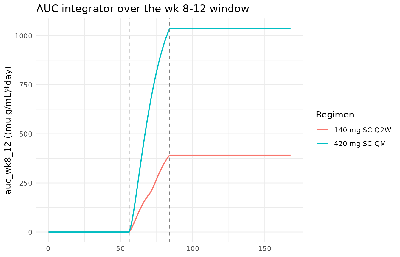
AUC accumulation inside the week-8-12 window (top) and the resulting LDLC algebraic observable (bottom). The LDLC trace is meaningful only at t >= 84 (vertical grey line); before then, the AUC window is still accumulating and the algebraic value is not the paper’s predicted response.
print(ldlc_panel)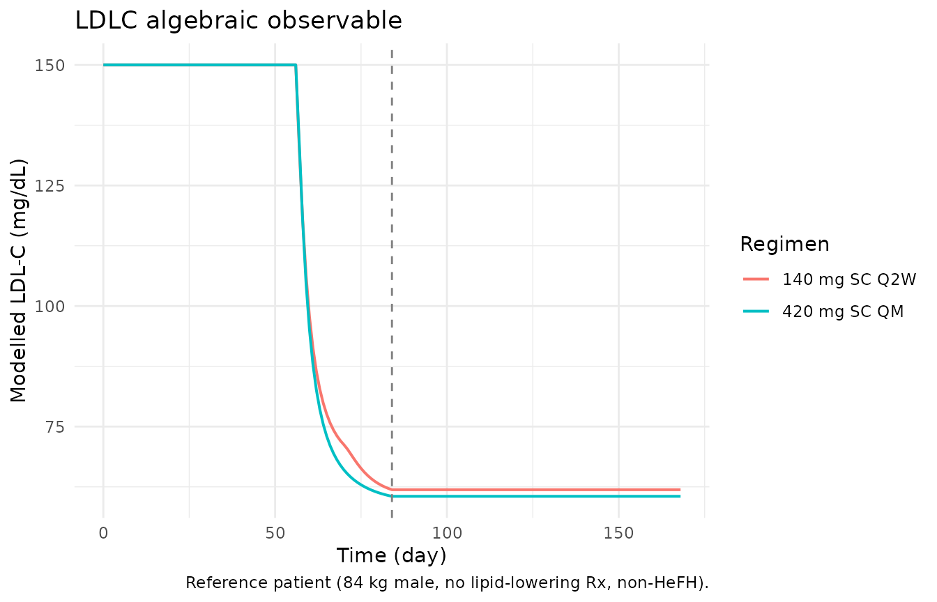
AUC accumulation inside the week-8-12 window (top) and the resulting LDLC algebraic observable (bottom). The LDLC trace is meaningful only at t >= 84 (vertical grey line); before then, the AUC window is still accumulating and the algebraic value is not the paper’s predicted response.
Comparison against the paper’s predicted maximal response
The paper reports that the model-predicted maximal LDL-C reduction at
the mean of weeks 10 and 12 is 99.7 mg/dL from a typical baseline of 150
mg/dL (approximately a 66% reduction), achieved as the AUC predictor
approaches infinity. At the two commercial regimens, the paper’s
reference-patient prediction is approximately 80% of the maximal
reduction. The next chunk extracts the modelled LDLC at day
84 (the canonical “mean of weeks 10 and 12” time point in the model) and
compares against this expectation.
sim_day84 <- sim_ldlc |>
  dplyr::filter(time == 84) |>
  dplyr::select(regimen, auc_wk8_12, LDLC)

ldlc_cmp <- sim_day84 |>
  dplyr::mutate(
    baseline_ldlc_mgdL   = 150,
    pct_reduction        = round(100 * (baseline_ldlc_mgdL - LDLC) / baseline_ldlc_mgdL, 1),
    pct_of_maximal       = round(100 * (baseline_ldlc_mgdL - LDLC) / 99.7,  1)
  )

knitr::kable(ldlc_cmp,
caption = "Modelled LDL-C at day 84 (mean week-10-12 surrogate) and percentage of the published maximal reduction (99.7 mg/dL).")| regimen | auc_wk8_12 | LDLC | baseline_ldlc_mgdL | pct_reduction | pct_of_maximal |
|---|---|---|---|---|---|
| 140 mg SC Q2W | 391.0453 | 61.90232 | 150 | 58.7 | 88.4 |
| 140 mg SC Q2W | 391.0453 | 61.90232 | 150 | 58.7 | 88.4 |
| 420 mg SC QM | 1035.7316 | 60.53190 | 150 | 59.6 | 89.7 |
| 420 mg SC QM | 1035.7316 | 60.53190 | 150 | 59.6 | 89.7 |
Both regimens should land near the paper’s 80%-of-maximal target,
with the QM arm sitting slightly farther from the asymptote than the Q2W
arm because of the regimen multiplier on EC50
(reg_qm = 2.30).
Assumptions and deviations
-
IIV block matrix approximated as diagonal.
Kuchimanchi 2018 states that CL, V, and Vmax share a
full-block variance matrix and refers the reader to “Table 4” for the
inter-parameter correlations. However, the paper’s Table 4 is the
exposure-response model parameter table and does not list the
population-PK omega-block correlations; the correlations are not
published anywhere in the article or supplement. Both model files
therefore encode independent diagonal IIV on CL, V, and Vmax.
This understates the individual-level covariance structure relative to
the published fit (in particular the high CL-Vmax correlation
that the paper calls out as influencing body-weight covariate-effect
precision) but has no effect on typical-value
(
rxode2::zeroRe()) simulation or on population-level summaries. -
Exposure-response model represented as a coupled rxode2
simulator. Kuchimanchi 2018 fit the Emax
relationship as a cross-sectional algebraic model with
individual-predicted AUCwk8-12 from the popPK fit as the
predictor. The packaged
Kuchimanchi_2018_evolocumab_ldlcrebuilds the same algebraic relationship inside an rxode2 model by carrying an extraauc_wk8_12state that integrates Cc only in the 56-84-day window. The numerical LDLC value att = 84matches what the paper’s equation produces for a given AUCwk8-12, but the intermediate values fort < 84are not interpretable as the paper’s E-R prediction. - Molecular weight used to convert between the paper’s target-unit scale (nM) and the model’s concentration scale (µg/mL) is 141 800 g/mol (evolocumab, FDA-approved Repatha label). The paper does not state the molecular weight explicitly; the same value reproduces the paper’s 5.9 nM ≈ 425 ng/mL reference-PCSK9 relationship within rounding when the PCSK9 molecular weight (~72 kDa) is applied to PCSK9.
- Reference patient characteristics used in the virtual cohort are the Methods-section reference definition: 84 kg male, not on lipid-lowering medication, baseline PCSK9 = 425 ng/mL. Body weight distribution and PCSK9 distribution in the broader trial population (which shifts observed mean Cmax slightly relative to the reference patient) are not reproduced in this typical-value simulation.
-
Time-fixed covariates. All covariates in the
PK-only model (
WT,SEXF,CONMED_STATIN_MONO,CONMED_EZE,PCSK9) and the joint PK + LDL-C model (the same five plusDIS_HEFHandREGI_QM) are treated as baseline time-fixed. Kuchimanchi 2018’s dataset used baseline values for these covariates; concomitant-medication status was required to be stable (>4 weeks of administration before study day 1) in the exposure-response analysis, though the popPK analysis used any duration of administration. -
REGI_QMis a per-subject covariate, not a derived quantity. The joint PK + LDL-C model carries the canonical covariateREGI_QM(1 = QM dosing, 0 = Q2W) as a per-subject input. The model does not infer the regimen from the dosing-interval column; users must set REGI_QM explicitly to match the regimen they are simulating. Mismatched values (e.g., REGI_QM = 1 with a 14-day dosing interval) produce a valid simulation but do not correspond to the paper’s E-R fit. -
auc_wk8_12window discipline. The LDLC algebraic observable is only meaningful att >= 84(end of the AUC integration window). Observation events placed before day 84 will produce LDLC values that reflect an only-partially-accumulated AUC and do not correspond to the paper’s E-R prediction. For population summaries the canonical observation time is day 84 (“mean of weeks 10 and 12” surrogate, per Methods).