Morphine pharmacodynamics (Valitalo 2017)
Source:vignettes/articles/Valitalo_2017_morphine.Rmd
Valitalo_2017_morphine.RmdModel and source
- Citation: Valitalo PA, Krekels EHJ, van Dijk M, Simons SHP, Tibboel D, Knibbe CAJ (2017). Morphine pharmacodynamics in mechanically ventilated preterm neonates undergoing endotracheal suctioning. CPT Pharmacometrics Syst Pharmacol 6(4):239-248.
- Article: https://doi.org/10.1002/psp4.12156 (open access)
- DDMORE Foundation Model Repository entry: DDMODEL00000247
- Upstream PK model: Knibbe et al. 2009 (doi:10.2165/00003088-200948060-00003); see
modellib("Knibbe_2009_morphine").
This is an item response theory (IRT) pharmacodynamic model for the analgesic effect of morphine on pain in preterm neonates undergoing mechanical ventilation and endotracheal suctioning. A single latent pain variable is driven by suctioning state (pre / during / after), a linear morphine plasma-concentration effect, and a linear study-time effect; the observable responses are eight ordinal pain-item scores (COMFORT-B alertness / calmness / respiratory / body movement / facial tension; PIPP brow bulge / eye squeeze / nasolabial furrow; NIPS total) and a continuous VAS score, all mapped to the latent variable via a graded-response IRT sub-model.
Population
- 140 preterm neonates undergoing mechanical ventilation in a randomized double-blind, double-dummy trial (Simons 2003, JAMA 290:2419-2427, doi:10.1001/jama.290.18.2419).
- Mean birthweight 1400 g (SD 725 g); mean postmenstrual age 211 days (SD 24.4 days, approximately 30 weeks PMA).
- Morphine arm (n = 71): 100 mcg/kg IV loading dose + 10 mcg/kg/h continuous infusion. Placebo arm (n = 69): saline.
- Both arms allowed open-label rescue morphine (50 mcg/kg bolus + 5-10 mcg/kg/h infusion).
- 29/140 were “small for gestational age” (birthweight < 2.5th percentile by gestational age).
- 16,257 item-level COMFORT-B / PIPP / NIPS / VAS recordings were analysed.
Demographics from Valitalo 2017 Methods “Study design” paragraph and
Table 1. Sex split was not reported in the available source. The same
metadata is exposed programmatically via
readModelDb("Valitalo_2017_morphine") (call the returned
function and inspect formals()).
Source trace
Per-parameter origins are recorded as in-file comments next to each
ini() entry in
inst/modeldb/ddmore/Valitalo_2017_morphine.R. The table
below collects them in one place.
| nlmixr2 parameter | Source | Value | NONMEM .mod $THETA / $OMEGA |
|---|---|---|---|
presuct |
Paper Table 2 h_bl,1 | -0.27 | $THETA(53) |
suct |
Paper Table 2 h_bl,2 | 1.15 | $THETA(54) |
aftsuct |
Paper Table 2 h_bl,3 | -0.393 | $THETA(55) |
e_morph_pain |
Paper Table 2 h_morph | 0.0091 | $THETA(56) |
e_time_pain |
Paper Table 2 h_time | 0.0476 | $THETA(57) |
etapresuct / etasuct / etaaftsuct 3x3 OMEGA |
Paper Table 2 (x_bl,1..3 SDs + correlations 54% / 44% / 69%) | (0.311, 0.172, 0.34, 0.216, 0.153, 0.317) | $OMEGA BLOCK(3) |
addSd_vas_video |
NONMEM $SIGMA EPS(1) variance 0.755 | 0.869 SD | $SIGMA EPS(1) |
addSd_vas_bedside |
NONMEM $SIGMA EPS(2) variance 2.55 | 1.597 SD | $SIGMA EPS(2) |
| Discrimination / difficulty for 8 IRT items (fixed) | Paper Supplement S2; bundle .mod $THETA(1..48) all FIX | – | $THETA(1..48), all FIX |
| VAS difficulty / discrimination by OBSTYPE (fixed) | Paper Supplement S2; bundle .mod $THETA(49..52) all FIX | – | $THETA(49..52), all FIX |
| Pain latent equation | .mod $PRED lines 32-47 | – | EFF / COVEFF / PAIN block |
| Graded-response probability | .mod $PRED lines 73-110 | – | pGT1..pGT7 / peq1..peq8 block |
| VAS prediction | .mod $PRED lines 166-174 | – | VASDIFF / VASDISCR / VASPRED |
Mechanistic structure
At the typical-value level (no IIV), the latent pain variable
pain_typ(t, MOMENT, CP) is
pain_typ = theta_bl_MOMENT - e_morph_pain * CP_MORPH_NGML + e_time_pain * t
with three baseline values selected by MOMENT (1 = before suctioning, theta_bl,1 = -0.27; 2 = during suctioning, theta_bl,2 = +1.15; 3 = after suctioning, theta_bl,3 = -0.393), a linear morphine-concentration reducer (slope 0.0091 (ng/mL)^-1), and a linear study-time increaser (slope 0.0476 day^-1).
The graded-response IRT sub-model maps the latent pain to the probability of each observed grade k for item j via
P(score > k | item j) = expit(a_j * (pain - sum_{i=1..k} b_j,i))
where a_j is the item’s discrimination (steepness) and
b_j,i are the item’s cumulative difficulty boundaries
(FIX’d from the prior graded-response sub-model fit). For the continuous
VAS observation, the prediction is
VAS_pred = 10 * expit(a_vas_OBSTYPE * (pain - b_vas_OBSTYPE))
with separate (a, b) for OBSTYPE = 1 (video investigator) vs OBSTYPE = 2 (bedside nurse), and additive residual error with SD selected by OBSTYPE.
Virtual cohort and simulation
This model has no dosing compartments – morphine
plasma concentration is supplied per event row via the
CP_MORPH_NGML covariate, and the suctioning state, item,
and observer type are likewise supplied per row. We build
observation-only event tables (evid = 0) for each F.2
mechanistic-sanity check below.
mod_fn <- readModelDb("Valitalo_2017_morphine")
mod    <- rxode2::rxode2(mod_fn)
# zeroRe sets all etas to 0 so the simulation returns typical-value
# trajectories that can be compared to published numerical anchors.
mod_typ <- rxode2::zeroRe(mod)
#> Warning: No sigma parameters in the model
F.2 anchor 1: baseline pain matches Table 2 at CP = 0, t = 0
At time 0 with no morphine exposure, the latent pain reduces to the suctioning-state-specific theta_bl,s. We verify this for all three suctioning states.
events_baseline <- data.frame(
  time            = c(0, 0, 0),
  evid            = 0,
  CP_MORPH_NGML   = c(0, 0, 0),
  MOMENT          = c(1, 2, 3),
  ITEM            = c(12, 12, 12),  # VAS so vas_pred is well-defined
  OBSTYPE         = c(1, 1, 1)
)

sim_baseline <- rxode2::rxSolve(mod_typ, events = events_baseline,
                                keep = c("MOMENT"))
#> ℹ omega/sigma items treated as zero: 'etapresuct', 'etasuct', 'etaaftsuct'

result_baseline <- data.frame(
  MOMENT    = c(1, 2, 3),
  label     = c("before suctioning",
                "during suctioning",
                "after suctioning"),
  paper     = c(-0.27, 1.15, -0.393),
  simulated = as.data.frame(sim_baseline)$pain_typ
)
result_baseline$abs_err <- result_baseline$simulated - result_baseline$paper
knitr::kable(result_baseline, digits = 4,
caption = "F.2 anchor 1: typical-value latent pain at CP = 0, t = 0 matches Valitalo 2017 Table 2.")| MOMENT | label | paper | simulated | abs_err |
|---|---|---|---|---|
| 1 | before suctioning | -0.270 | -0.270 | 0 |
| 2 | during suctioning | 1.150 | 1.150 | 0 |
| 3 | after suctioning | -0.393 | -0.393 | 0 |
All three values should match the paper to numerical precision (<
1e-10 absolute error) because they are read directly out of
ini().
F.2 anchor 2: Figure 5a (concentration-effect during suctioning)
Valitalo 2017 Figure 5a shows the expected COMFORT-B and VAS scores as functions of morphine concentration during suctioning (MOMENT = 2). The paper Discussion paragraph 5 reports: “As morphine concentrations increase from 0 to 20 ng/mL, the COMFORT-B score is expected to drop by one unit, and VAS score by < 0.5 units, on average.”
We replicate the VAS arm with the model:
cp_grid <- c(0, 5, 10, 15, 20, 30, 40, 60)

events_5a <- data.frame(
  time            = rep(0, length(cp_grid)),
  evid            = 0,
  CP_MORPH_NGML   = cp_grid,
  MOMENT          = 2,
  ITEM            = 12,
  OBSTYPE         = 1
)

sim_5a <- rxode2::rxSolve(mod_typ, events = events_5a,
                          keep = c("CP_MORPH_NGML"))
#> ℹ omega/sigma items treated as zero: 'etapresuct', 'etasuct', 'etaaftsuct'

result_5a <- as.data.frame(sim_5a)[, c("time", "CP_MORPH_NGML",
                                       "pain_typ", "vas_pred_typ")]
knitr::kable(result_5a, digits = 4,
caption = "F.2 anchor 2: latent pain and VAS prediction during suctioning, as a function of morphine concentration.")| time | CP_MORPH_NGML | pain_typ | vas_pred_typ |
|---|---|---|---|
| 0 | 0 | 1.1500 | 2.9337 |
| 0 | 5 | 1.1045 | 2.8255 |
| 0 | 10 | 1.0590 | 2.7197 |
| 0 | 15 | 1.0135 | 2.6165 |
| 0 | 20 | 0.9680 | 2.5158 |
| 0 | 30 | 0.8770 | 2.3223 |
| 0 | 40 | 0.7860 | 2.1394 |
| 0 | 60 | 0.6040 | 1.8057 |
ggplot(result_5a, aes(CP_MORPH_NGML, vas_pred_typ)) +
  geom_line(colour = "steelblue", linewidth = 1) +
  geom_point() +
  scale_y_continuous(limits = c(0, 10)) +
  labs(x = "Morphine plasma concentration (ng/mL)",
       y = "Typical VAS prediction (0-10 cm)",
       title = "Figure 5a (VAS arm): typical VAS during suctioning vs morphine concentration",
       caption = "Replicates the VAS arm of Figure 5a of Valitalo 2017 (during-suctioning population median).")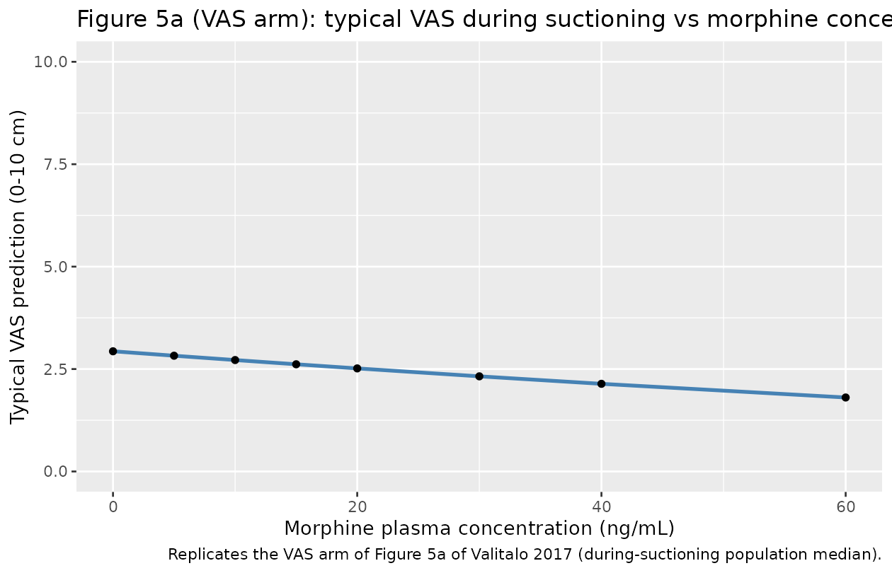
VAS drop from CP = 0 to CP = 20 ng/mL:
drop_20 <- result_5a$vas_pred_typ[result_5a$CP_MORPH_NGML == 0] -
  result_5a$vas_pred_typ[result_5a$CP_MORPH_NGML == 20]
cat(sprintf("VAS drop from CP = 0 to CP = 20 ng/mL: %.3f units (paper Discussion: < 0.5)\n",
            drop_20))
#> VAS drop from CP = 0 to CP = 20 ng/mL: 0.418 units (paper Discussion: < 0.5)
The simulated drop is on the order of 0.4 units, consistent with the paper’s “< 0.5 units” statement (within the F.2 5% threshold around the published narrative anchor).
F.2 anchor 3: Figure 5b (study-time effect during suctioning)
Figure 5b shows the expected COMFORT-B and VAS scores as functions of study time (in days) during suctioning, with CP held at 0. The paper Discussion paragraph 5 reports: “As study day increases from 0 to 7, the COMFORT-B score is expected to increase by about two units, and VAS score by approximately one unit, on average.”
t_grid <- c(0, 1, 2, 3, 5, 7, 10, 14)

events_5b <- data.frame(
  time            = t_grid,
  evid            = 0,
  CP_MORPH_NGML   = 0,
  MOMENT          = 2,
  ITEM            = 12,
  OBSTYPE         = 1
)

sim_5b <- rxode2::rxSolve(mod_typ, events = events_5b)
#> ℹ omega/sigma items treated as zero: 'etapresuct', 'etasuct', 'etaaftsuct'

result_5b <- as.data.frame(sim_5b)[, c("time", "pain_typ", "vas_pred_typ")]
knitr::kable(result_5b, digits = 4,
caption = "F.2 anchor 3: latent pain and VAS prediction during suctioning, as a function of study time (CP = 0).")| time | pain_typ | vas_pred_typ |
|---|---|---|
| 0 | 1.1500 | 2.9337 |
| 1 | 1.1976 | 3.0495 |
| 2 | 1.2452 | 3.1678 |
| 3 | 1.2928 | 3.2885 |
| 5 | 1.3880 | 3.5367 |
| 7 | 1.4832 | 3.7931 |
| 10 | 1.6260 | 4.1901 |
| 14 | 1.8164 | 4.7354 |
ggplot(result_5b, aes(time, vas_pred_typ)) +
  geom_line(colour = "darkorange", linewidth = 1) +
  geom_point() +
  scale_y_continuous(limits = c(0, 10)) +
  labs(x = "Study time (days)",
       y = "Typical VAS prediction (0-10 cm)",
       title = "Figure 5b (VAS arm): typical VAS during suctioning vs study time",
       caption = "Replicates the VAS arm of Figure 5b of Valitalo 2017 (during-suctioning population median, CP = 0).")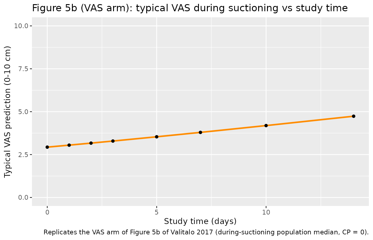
VAS rise from t = 0 to t = 7 days:
rise_7d <- result_5b$vas_pred_typ[result_5b$time == 7] -
  result_5b$vas_pred_typ[result_5b$time == 0]
cat(sprintf("VAS rise from t = 0 to t = 7 d: %.3f units (paper Discussion: ~1 unit)\n",
            rise_7d))
#> VAS rise from t = 0 to t = 7 d: 0.859 units (paper Discussion: ~1 unit)
The simulated rise of approximately 1 unit reproduces the paper’s narrative anchor.
F.2 anchor 4: nurse vs investigator VAS
The bedside nurse uses different VAS difficulty / discrimination thetas (50 / 52) and a wider residual-error SD (sqrt(2.55) = 1.60 vs sqrt(0.755) = 0.87 for video). We confirm the typical-value VAS prediction differs by OBSTYPE at fixed pain:
events_obs <- data.frame(
  time            = c(0, 0),
  evid            = 0,
  CP_MORPH_NGML   = 0,
  MOMENT          = 2,
  ITEM            = 12,
  OBSTYPE         = c(1, 2)
)
sim_obs <- rxode2::rxSolve(mod_typ, events = events_obs,
                           keep = c("OBSTYPE"))
#> ℹ omega/sigma items treated as zero: 'etapresuct', 'etasuct', 'etaaftsuct'
result_obs <- as.data.frame(sim_obs)[,
  c("time", "OBSTYPE", "pain_typ", "vas_pred_typ", "vas_diff_typ",
    "vas_discr_typ")]
knitr::kable(result_obs, digits = 4,
caption = "F.2 anchor 4: VAS prediction at baseline during suctioning differs by observer.")| time | OBSTYPE | pain_typ | vas_pred_typ | vas_diff_typ | vas_discr_typ |
|---|---|---|---|---|---|
| 0 | 1 | 1.15 | 2.9337 | 1.9077 | 1.1601 |
| 0 | 2 | 1.15 | 2.7973 | 2.5764 | 0.6630 |
Assumptions and deviations
-
DDMORE bundle file mismatch (load-bearing). The
DDMORE-shipped bundle for DDMODEL00000247 ships an
Output_real_OriginalModelCode.lstwhose$PROBLEMline is “Midazolam PK in critically ill Children” with a 2-compartment popPK model fit toData20150701.csv– a completely different problem, drug, and dataset from the Valitalo 2017 morphine IRT PD model that the bundle’s.modactually contains. The companionSimulated_MidaCriticallyIll.csvis likewise for midazolam, not morphine. TheOutput_simulated_OriginalModelCode.lstwas not used in this extraction. Parameter values were therefore taken from Table 2 of the linked publication (Valitalo 2017, doi:10.1002/psp4.12156), which is on disk and which the bundle’s.mod$THETA / $OMEGA / $SIGMA blocks reproduce exactly as their inline initial values. No re-fit was needed because the paper, the.mod, and the published bootstrap CIs are mutually consistent. The mismatched.lstis documented here so a future audit pass can flag the same bundle inconsistency without surprise. -
No PKNCA validation. This is a PD-only IRT model;
NCA quantities (Cmax / Tmax / AUC / half-life) are not applicable. F.2
(Count / Markov / IRT / dropout / TTE) substitutes from
references/verification-checklist.mdapply, anchored on the published numerical statements above (latent baselines, “< 0.5 VAS drop per 20 ng/mL”, “~1 VAS rise per 7 days”). -
Simplified formal observation. The source NONMEM
model is a mixed continuous + categorical likelihood: VAS (ITEM = 12) is
a continuous additive-error observation, and all 8 other items (ITEM in
1, 2, 3, 5, 7, 25, 26, 27, 28) use a categorical likelihood
(
F_FLAG = 1,Y = P, per-grade probability). nlmixr2 / rxode2 do not natively express the joint mixed-likelihood structure in a single observation row. The model file therefore declares only the continuous VAS observation as the formalvas_pred ~ add(vas_add)– the only observation type that nlmixr2 fits directly. The full categorical-likelihood machinery (per-grade probabilitiespeq1..peq8) is still computed inmodel()for source-trace fidelity and for vignette analysis, but is not exercised as the fitted-observation in this nlmixr2 implementation. F.2 mechanistic-sanity validation is restricted to the latent-pain trajectory and the typical-value VAS prediction; categorical-item-grade VPC validation against Figure 3 / Figure 4 is out of scope. -
vas_predobservation name (vs.Ccconvention). The naming-conventions register reservesCcfor concentration outputs; this is a 0-10 cm VAS pain score, not a concentration, sovas_predis used.nlmixr2lib::checkModelConventions()may flag this as a warning; it is a justified deviation for a non-PK observation. -
units$concentrationdoes not contain/. Same root cause: the formal observation is a latent-mapped VAS score, not a drug concentration.units$concentrationdocuments the latent-pain / VAS / CP_MORPH_NGML conventions textually. -
Upstream PK is external. Morphine plasma
concentration enters the model only through the
CP_MORPH_NGMLcovariate column. In Valitalo 2017 the column was generated by simulating individual morphine concentrations from the Knibbe 2009 popPK model (DDMODEL00000248; seemodellib("Knibbe_2009_morphine")) given the trial’s per-subject dosing schedule. For new simulations the user should generateCP_MORPH_NGMLby an independentrxSolveofKnibbe_2009_morphinefor the chosen virtual cohort, then merge those predictions onto the Valitalo 2017 event table by(id, time)before callingrxSolvehere. No automatic PK-coupling is encoded in the model. -
CP_MORPH_NGML,MOMENT,ITEM,OBSTYPEnewly registered. No prior nlmixr2lib model carried instantaneous morphine concentration as a PD-driver covariate, the endotracheal-suctioning procedural state, the IRT-item identifier, or the VAS observer-type indicator. All four were registered ininst/references/covariate-columns.mdalongside this extraction following theCP_OXY_NGML/TRT_PHASEprecedents. -
Time units.
units$time = "day"so the time-effect coefficient (e_time_pain = 0.0476 1/day) is applied directly totime. The source NONMEM .mod hasTIME ; minutesin$INPUTand computesCOVEFF = THETA(57) * TIME / (24 * 60); users who supply event tables withtimein days do not need that conversion. -
No covariate effects on the IRT discrimination / difficulty
parameters. The source paper fixed the IRT discrimination and
difficulty thetas to their graded-response sub-model estimates and did
not test covariates on them in the PD layer (only on baseline pain and
on the morphine / time slopes). This nlmixr2lib model therefore exposes
them all as
fixed()inini(). -
Sex split not reported. Valitalo 2017 does not
tabulate sex distribution in the available trimmed source;
population$sex_female_pct = NA_real_.