Model and source
Citation: Wu F, Krishna G, Surapaneni S. Physiologically based pharmacokinetic modeling to assess metabolic drug-drug interaction risks and inform the drug label for fedratinib. Cancer Chemother Pharmacol. 2020;86(4):461-473. doi:10.1007/s00280-020-04131-y
Description: Two-compartment oral PK model of fedratinib with first-order absorption, fitted naive-pooled to mean plasma profiles after a single 500 mg dose in healthy volunteers (Wu 2020, Supplemental Material SM3). This is the compartmental fit the authors used to seed the distribution inputs of their Simcyp minimal-PBPK DDI model; the PBPK layer itself is not included. Typical-value model: no IIV and no residual-error magnitude were reported.
PubMed Central: https://www.ncbi.nlm.nih.gov/pmc/articles/PMC7515950/
Electronic supplementary material (ESM 1, Supplemental Materials SM1-SM12): distributed with the open-access article.
Wu 2020 built a physiologically based pharmacokinetic (PBPK) drug-drug interaction model of the JAK2 inhibitor fedratinib in Simcyp V17R1 and used it to support the fedratinib label (dose reduction to 200 mg QD with a strong CYP3A4 inhibitor). The Simcyp model uses the platform’s minimal-PBPK distribution model with a single adjusting compartment, enzyme-kinetic hepatic clearance scaled from recombinant CYP intrinsic clearances, and mechanism-based inhibition and induction of CYP3A4 by fedratinib itself.
To seed the minimal-PBPK distribution inputs, the authors first fitted a conventional two-compartment model with first-order absorption to mean plasma profiles from four healthy-volunteer studies of a single 500 mg dose (Supplemental Material SM3). That compartmental model is what this package provides.
Why the PBPK model itself is not included. The
Simcyp model’s clearance, auto-inhibition and auto-induction terms act
on hepatic and intestinal CYP enzyme pools whose abundances, microsomal
protein per gram of liver, liver weight, enzyme degradation rates and
intestinal physiology come from the Simcyp “Healthy Volunteers” and
“Cancer” population library files, which the authors used “without
further modification” and which are not published in the paper or its
supplement. The compound-specific inputs (SM4) are printed in full, but
without the platform’s system parameters they cannot be turned into a
standalone ODE system. A population PK model of fedratinib in patients
with myelofibrosis, polycythemia vera and essential thrombocythemia is
available as Ogasawara_2019_fedratinib.
Population
Mean plasma concentration-time profiles pooled from four healthy-volunteer studies (TDU12620 single ascending dose, BDR12462 tablet-vs-capsule bioequivalence, FED12258 and ALI13451 food effect), all given single 500 mg doses (Wu 2020 SM3). Three of the four studies are described as enrolling healthy male subjects (SM1 Table 1); the fourth (BDR12462) does not state sex. The number of subjects contributing to the mean profiles is not reported. The fit used the Phoenix NLME ‘naive pooled’ algorithm, so no between-subject variability was estimated.
The mean profiles came from studies TDU12620 (single ascending doses in healthy men), BDR12462 (500 mg tablet vs capsule bioequivalence), FED12258 and ALI13451 (food effect on a single 500 mg dose in healthy men); the study list is SM1 Table 1 and the pooling is described in SM3. Neither the number of subjects nor the demographics of the pooled set are reported.
Source trace
| Model element | Value | Source location |
|---|---|---|
| Structure: 2-compartment, first-order absorption, additive error | – | SM3 text |
lka (ka) |
0.221 1/h | SM3 compartmental PK parameter table |
lcl (CL/F) |
27.2 L/h | SM3 compartmental PK parameter table |
lvc (V/F) |
107 L | SM3 compartmental PK parameter table; restated in SM2 “Distribution Parameters” |
lq (CL2/F) |
30.8 L/h | SM3 compartmental PK parameter table; restated in SM2 |
lvp (V2/F) |
797 L | SM3 compartmental PK parameter table; restated in SM2 |
addSd |
fixed 0 | SM3 names an additive error model; no magnitude printed |
| IIV | none | SM3: Phoenix NLME “naive pooled” algorithm |
Cc = 1000 * central / vc |
ng/mL | unit conversion (mg / L to ng/mL, the units of the paper’s exposure tables) |
| Derived minimal-PBPK inputs Vss, Vsac, Q | 4.1 L/kg, 3.5 L/kg, 11 L/h | SM2 Eqs (1)-(3) with F = 0.36 and 81 kg; SM2 Table 1 and SM4 |
| Observed single-dose exposures | see comparison table | SM6 Table (healthy subjects, 300 and 500 mg single dose); main-text Table 1 (INT12893, 300 mg alone) |
Internal consistency with the published PBPK inputs
SM2 converts the compartmental estimates into the Simcyp minimal-PBPK
inputs with Eqs (1)-(3): Vss = (V/F + V2/F) * F,
Vsac = V2/F * F and Q = CL2/F * F, using
F = 0.36 and a body weight of 81 kg for volumes per kg.
Recomputing the three inputs from this model’s ini() values
reproduces the printed values, which checks the transcription of
V/F, V2/F and CL2/F against a
second, independent place in the supplement.
p <- ui$theta
f_sm2 <- 0.36
wt_sm2 <- 81
recomputed <- c(
  Vss_L_per_kg = (exp(p[["lvc"]]) + exp(p[["lvp"]])) * f_sm2 / wt_sm2,
  Vsac_L_per_kg = exp(p[["lvp"]]) * f_sm2 / wt_sm2,
  Q_L_per_h = exp(p[["lq"]]) * f_sm2
)
printed <- c(Vss_L_per_kg = 4.1, Vsac_L_per_kg = 3.5, Q_L_per_h = 11)

tibble::tibble(
  Input = names(printed),
  Printed = printed,
  Recomputed = signif(recomputed, 3),
  `Difference (%)` = round(100 * (recomputed / printed - 1), 1)
) |>
knitr::kable(caption = "Simcyp minimal-PBPK inputs recomputed from the SM3 estimates (SM2 Eqs 1-3).")| Input | Printed | Recomputed | Difference (%) |
|---|---|---|---|
| Vss_L_per_kg | 4.1 | 4.02 | -2.0 |
| Vsac_L_per_kg | 3.5 | 3.54 | 1.2 |
| Q_L_per_h | 11.0 | 11.10 | 0.8 |
Simulation
The model has no between-subject variability, so a single deterministic solve per dose gives the typical profile. Single oral doses of 300 mg and 500 mg are simulated, matching the healthy-volunteer single-dose scenarios the paper reports.
doses <- c(300, 500)
obs_times <- sort(unique(c(seq(0, 24, by = 0.1), seq(24.5, 96, by = 0.5), seq(98, 720, by = 2))))

ev <- dplyr::bind_rows(
  tibble::tibble(id = seq_along(doses), time = 0, amt = doses, evid = 1L, cmt = "depot"),
  tidyr::expand_grid(id = seq_along(doses), time = obs_times) |>
    dplyr::mutate(amt = NA_real_, evid = 0L, cmt = "central")
) |>
  dplyr::mutate(treatment = paste0(doses[id], " mg")) |>
  dplyr::arrange(id, time, dplyr::desc(evid))

sim <- rxode2::rxSolve(mod, events = ev, keep = "treatment") |>
  as.data.frame()
#> Warning: multi-subject simulation without without 'omega'

stopifnot(nrow(sim) == length(doses) * length(obs_times))
ggplot(dplyr::filter(sim, time <= 168), aes(time, Cc, colour = treatment)) +
  geom_line() +
  scale_y_log10() +
  labs(x = "Time after dose (h)", y = "Fedratinib (ng/mL)", colour = "Single dose") +
  theme_bw()
#> Warning in scale_y_log10(): log-10 transformation introduced infinite values.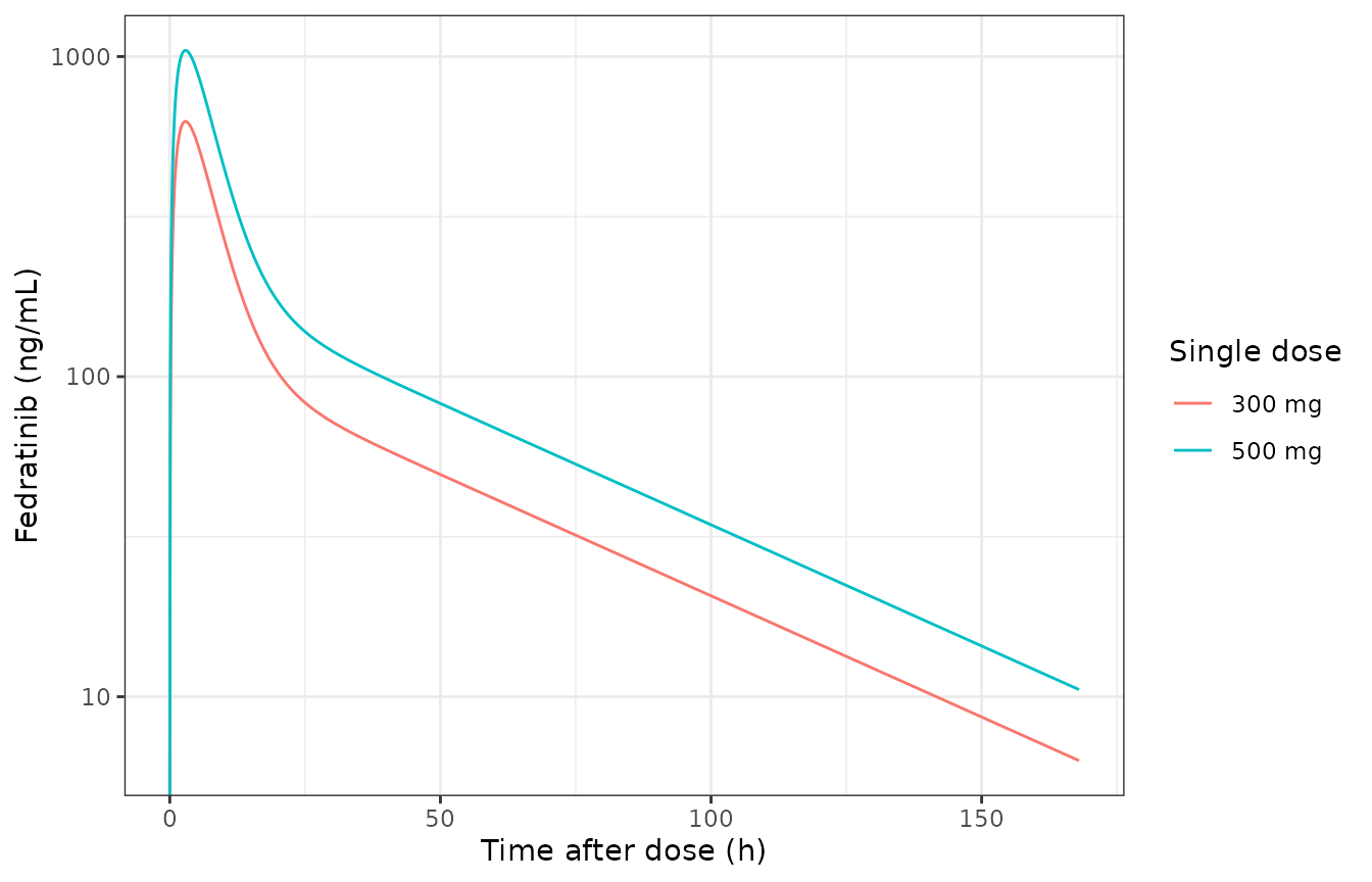
Typical fedratinib plasma concentration after a single oral dose (compare with the healthy-volunteer single-dose panels a and b of Wu 2020 Figure 2, which show the Simcyp predictions and the observed mean data).
NCA with PKNCA
sim_nca <- sim |>
  dplyr::filter(!is.na(Cc)) |>
  dplyr::select(id, time, Cc, treatment)

# Guarantee a time = 0 row per subject (pre-dose Cc = 0 for an oral dose).
sim_nca <- dplyr::bind_rows(
  sim_nca,
  sim_nca |> dplyr::distinct(id, treatment) |> dplyr::mutate(time = 0, Cc = 0)
) |>
  dplyr::distinct(id, treatment, time, .keep_all = TRUE) |>
  dplyr::arrange(id, treatment, time)

dose_df <- ev |>
  dplyr::filter(evid == 1L) |>
  dplyr::select(id, time, amt, treatment)

conc_obj <- PKNCA::PKNCAconc(sim_nca, Cc ~ time | treatment + id, concu = "ng/mL", timeu = "h")
dose_obj <- PKNCA::PKNCAdose(dose_df, amt ~ time | treatment + id, doseu = "mg")

intervals <- data.frame(
  start = 0, end = Inf,
  cmax = TRUE, tmax = TRUE, aucinf.obs = TRUE, half.life = TRUE, cl.obs = TRUE
)

nca_res <- PKNCA::pk.nca(PKNCA::PKNCAdata(conc_obj, dose_obj, intervals = intervals))
nca_wide <- as.data.frame(nca_res$result) |>
  dplyr::select(treatment, PPTESTCD, PPORRES) |>
  tidyr::pivot_wider(names_from = PPTESTCD, values_from = PPORRES)

nca_wide |>
  dplyr::select(treatment, cmax, tmax, aucinf.obs, half.life) |>
  dplyr::rename(
    "Single dose" = treatment,
    "Cmax (ng/mL)" = cmax,
    "Tmax (h)" = tmax,
    "AUC0-inf (ng*h/mL)" = aucinf.obs,
    "t1/2 (h)" = half.life
  ) |>
knitr::kable(digits = 1, caption = "PKNCA results for the typical profile.")| Single dose | Cmax (ng/mL) | Tmax (h) | AUC0-inf (ng*h/mL) | t1/2 (h) |
|---|---|---|---|---|
| 300 mg | 627.1 | 2.9 | 11028.9 | 39.6 |
| 500 mg | 1045.1 | 2.9 | 18381.5 | 39.6 |
The model is linear with no variability, so
AUC0-inf = Dose / (CL/F) must hold exactly, up to the
trapezoidal error of the sampling grid. This is a check of the solve
against its own closed form, so a tight bound is appropriate.
auc_identity <- nca_wide |>
  dplyr::mutate(
    dose = as.numeric(sub(" mg", "", treatment)),
    expected = 1000 * dose / exp(p[["lcl"]]),
    pct_diff = 100 * (aucinf.obs / expected - 1)
  )
auc_identity |>
  dplyr::select(treatment, aucinf.obs, expected, pct_diff) |>
knitr::kable(digits = 2, caption = "AUC0-inf from PKNCA vs Dose / (CL/F).")| treatment | aucinf.obs | expected | pct_diff |
|---|---|---|---|
| 300 mg | 11028.87 | 11029.41 | 0 |
| 500 mg | 18381.45 | 18382.35 | 0 |
Comparison against the published observed exposures
Wu 2020 reports observed single-dose exposures in healthy subjects in SM6 (300 mg and 500 mg, arithmetic mean with geometric mean in brackets) and, for 300 mg, in main-text Table 1 (the fedratinib-alone arm of the ketoconazole study INT12893). A typical-value profile is closest to a geometric mean, so the geometric means are used as the reference.
published <- tibble::tibble(
  treatment = c("300 mg", "500 mg"),
  cmax = c(497, 683), # SM6 table, healthy subjects single dose, GM
  aucinf.obs = c(6530, 13200) # SM6 table, healthy subjects single dose, GM
)

cmp <- nlmixr2lib::ncaComparisonTable(
  simulated = nca_res,
  reference = published,
  by = "treatment",
  params = c("cmax", "aucinf.obs"),
  units = c(cmax = "ng/mL", aucinf.obs = "ng*h/mL"),
  tolerance_pct = 20
)
knitr::kable(
  cmp,
  caption = paste(
    "Typical-value simulation vs observed geometric means in healthy subjects",
    "(Wu 2020 SM6). Rows marked with * differ by more than 20%."
  )
)| NCA parameter | treatment | Reference | Simulated | % diff |
|---|---|---|---|---|
| Cmax (ng/mL) | 300 mg | 497 | 627 | +26.2%* |
| Cmax (ng/mL) | 500 mg | 683 | 1050 | +53.0%* |
| AUC0-∞ (obs) (ng*h/mL) | 300 mg | 6530 | 11000 | +68.9%* |
| AUC0-∞ (obs) (ng*h/mL) | 500 mg | 13200 | 18400 | +39.3%* |
The typical profile over-predicts the observed geometric means:
AUC0-inf by about 69% at 300 mg and 39% at 500 mg, and Cmax by about 26%
and 53%. The AUC gap is a property of the published estimate, not of the
implementation: the AUC identity above shows the model returns exactly
Dose / (CL/F) with CL/F = 27.2 L/h, while the
observed geometric means imply a CL/F of about 46 L/h (300
mg) and 38 L/h (500 mg). The supplement is consistent with this. SM2
(“Metabolism Parameters”) reports that the compartmental
CL/F was only the starting value for Simcyp’s retrograde
clearance calculation and was then raised to 48 L/h so that the PBPK
model reproduced the observed dose-normalized AUC of 30
ngh/(mLmg), which corresponds to a CL/F of 33.3
L/h. The compartmental model was fitted to mean profiles pooled across
four studies (including food-effect and formulation arms), and the paper
does not say which subjects underlie the SM6 comparison rows. The
parameters are reproduced as published and have not been adjusted.
# Pin the size and sign of the discrepancy described above. The model is
# deterministic, so these ratios do not vary between runs or machines.
ratio <- nca_wide |>
  dplyr::inner_join(published, by = "treatment", suffix = c("_sim", "_obs")) |>
  dplyr::mutate(
    auc_ratio = aucinf.obs_sim / aucinf.obs_obs,
    cmax_ratio = cmax_sim / cmax_obs
  )
stopifnot(
  all(ratio$auc_ratio > 1.3 & ratio$auc_ratio < 1.8),
  all(ratio$cmax_ratio > 1.2 & ratio$cmax_ratio < 1.6)
)
Assumptions and deviations
- PBPK layer not implemented. Only the SM3 compartmental model is provided; the Simcyp minimal-PBPK DDI model depends on unpublished Simcyp population-library system parameters (see “Model and source”).
-
Residual error. SM3 states an additive error model
but gives no magnitude;
addSdis fixed at 0 so the model is a typical-value model. Simulations from it carry no residual noise. - No between-subject variability. The fit used the naive-pooled algorithm on mean profiles, which estimates none.
- Population. The number, sex and body size of the subjects behind the mean profiles are not reported. Three of the four studies enrolled healthy men only.
- Formulation and food. Two of the pooled studies were food-effect studies and one compared tablet with capsule. SM3 does not say which arms were included in the mean profiles; the model carries no food or formulation effect.
- Parameter table label. In the supplement the compartmental parameter table is cited as “Table 3 in Supplemental Material SM 3” in SM2; the values are also restated in the SM2 text (V/F 107 L, V2/F 797 L, CL2/F 30.8 L/h), which agree with the table.