Quinidine (Fattinger 1991)
Source:vignettes/articles/Fattinger_1991_quinidine.Rmd
Fattinger_1991_quinidine.RmdModel and source
- Citation: Fattinger K, Vozeh S, Ha HR, Borner M, Follath F (1991). Population pharmacokinetics of quinidine. Br J Clin Pharmacol 31(3):279-286. doi:10.1111/j.1365-2125.1991.tb05531.x.
- Description: Two-compartment population PK model for oral quinidine in adults treated for supraventricular or ventricular arrhythmias (Fattinger 1991). Zero-order absorption from the gastrointestinal tract with formulation-specific absorption duration: immediate-release quinidine sulphate (Chinidin sulfuricum) with a typical absorption duration of 1.37 h, and slow-release quinidine bisulphate (Kinidin duriles) with a typical absorption duration of 6.0 h and a 1.36-fold higher relative bioavailability versus quinidine sulphate. Apparent total clearance is the sum of a renal arm proportional to creatinine clearance (proportionality 0.0566 L/h per mL/min) and a non-renal arm of 12.6 L/h that is halved to 6.8 L/h in patients with severe heart failure or severe liver failure. Apparent central volume is 161 L. Inter-compartmental clearance Q is 12.6 L/h and peripheral volume V2 is 66.7 L. Inter-individual variability is assigned to total clearance (40.2% CV), central volume (75.6% CV), and the quinidine sulphate absorption duration (49.4% CV); residual variability is proportional (22% CV).
- Article: https://doi.org/10.1111/j.1365-2125.1991.tb05531.x
Population
Sixty adults (46 male, 14 female; median age 65.5 years, range 28-82; median body weight 70.5 kg, range 45-105 kg) treated for supraventricular or ventricular arrhythmias contributed 260 routine therapeutic-drug-monitoring serum quinidine concentrations to the model-development cohort (Fattinger 1991 Methods, page 280). Median creatinine clearance was 62.5 mL/min (range 17 to above 100 mL/min). The cohort spanned the full range of cardiac and hepatic status: severe heart failure n = 2, severe liver failure n = 3, moderate heart failure n = 20, mild heart failure n = 19, moderate liver dysfunction n = 22. Nine subjects received concomitant nifedipine; no nifedipine effect on quinidine PK was detected (Discussion, page 284).
The two oral formulations administered were Chinidin sulfuricum (quinidine sulphate, immediate-release; Siegfried) and Kinidin duriles (quinidine bisulphate, slow-release; Astra). The usual regimen was an initial 400 mg or 600 mg quinidine sulphate dose followed three hours later by 500 mg quinidine bisulphate twice or three times daily. Concentrations in the validation cohort of 30 separate patients (median CrCl 48.7 mL/min) lay within the 90% prediction interval 28/30 times (page 282).
The same information is available programmatically via
rxode2::rxode(readModelDb("Fattinger_1991_quinidine"))$population.
Source trace
The per-parameter origin is recorded as an in-file comment next to
each ini() entry in
inst/modeldb/specificDrugs/Fattinger_1991_quinidine.R. The
table below collects them in one place for review.
| Equation / parameter | Value | Source location |
|---|---|---|
e_crcl_cl_renal (log proportionality on CRCL) |
log(0.0566) | Fattinger 1991 Table 1: CL_renal = 0.0566 L/h per
mL/min |
lcl_nonren (non-renal CL, no severe HF/LF) |
log(12.6) | Fattinger 1991 Table 1: CL_nonrenal (no severe HF/LF) =
12.6 L/h |
e_dis_hf_or_lf_sev_cl_nonren (severe HF/LF
multiplicative shift) |
log(6.8 / 12.6) | Fattinger 1991 Table 1: CL_nonrenal (severe HF/LF) =
6.8 L/h (50% reduction relative to non-severe) |
lvc (apparent V1) |
log(161 L) | Fattinger 1991 Table 1: V1 = 161 L |
lq (Q, inter-compartmental CL) |
log(12.6 L/h) | Fattinger 1991 Table 1: Q = 12.6 L/h (footnote e
identifies Q as inter-compartmental clearance) |
lvp (apparent V2) |
log(66.7 L) | Fattinger 1991 Table 1: V2 = 66.7 L |
ldur_qs (zero-order absorption duration, QS) |
log(1.37 h) | Fattinger 1991 Table 1: t_max,QS = 1.37 h |
ldur_qbs (zero-order absorption duration, QBS) |
log(6.00 h) | Fattinger 1991 Table 1: t_max,QBS = 6.00 h |
lfdepot (log relative bioavailability QBS vs QS) |
log(1.36) | Fattinger 1991 Table 1: F = 1.36 (QS reference = 1,
assumed 100% per abstract item 3) |
etalcl (omega^2 on total CL) |
log(1 + 0.402^2) | Fattinger 1991 Table 1: IIV on CL = 40.2% CV |
etalvc (omega^2 on V1) |
log(1 + 0.756^2) | Fattinger 1991 Table 1: IIV on V1 = 75.6% CV |
etaldur_qs (omega^2 on QS duration) |
log(1 + 0.494^2) | Fattinger 1991 Table 1: IIV on t_max,QS = 49.4% CV |
propSd (proportional residual error) |
0.22 | Fattinger 1991 Table 1: sigma = 22% CV |
| Two-compartment zero-order absorption ODE | n/a | Fattinger 1991 Results, page 282: “A two compartment model with zero order absorption from the gastrointestinal tract was found to describe the data better than a one compartment model” |
| Salt-to-base stoichiometric factors | 0.829 (QS), 0.663 (QBS) | Fattinger 1991 Methods, page 280, citing Windholz 1983 |
| Modified Cockcroft-Gault for CRCL | CLcr = (150 - age) * WT / Scr (+10% males, -10% females) | Fattinger 1991 Methods, page 281, citing Cockcroft & Gault 1976 and Dettli 1983 |
Structural-parameter cross-check
The two-compartment hybrid rate constants derived from the structural typical-value parameters at the reference covariate state (CRCL = 100 mL/min, no severe HF/LF) exactly reproduce the half-lives reported on page 282 of Fattinger 1991.
tv_pars <- list(
  cl_renal = 0.0566,   # L/h per mL/min CRCL
  cl_nonren = 12.6,    # L/h non-severe
  v1 = 161,            # L (apparent Vc)
  q  = 12.6,           # L/h
  v2 = 66.7            # L (apparent Vp)
)
crcl_ref <- 100        # mL/min
cl_total <- tv_pars$cl_renal * crcl_ref + tv_pars$cl_nonren
ke  <- cl_total / tv_pars$v1
k12 <- tv_pars$q   / tv_pars$v1
k21 <- tv_pars$q   / tv_pars$v2
ssum <- ke + k12 + k21
disc <- sqrt(ssum^2 - 4 * ke * k21)
alpha <- (ssum + disc) / 2
beta  <- (ssum - disc) / 2

knitr::kable(
  data.frame(
    quantity = c(
      "Total apparent CL/F (L/h)",
      "t_half_alpha (h)",
      "t_half_beta  (h)",
      "Renal fraction at CRCL=100 mL/min"
    ),
    derived = c(
      sprintf("%.2f", cl_total),
      sprintf("%.2f", log(2) / alpha),
      sprintf("%.2f", log(2) / beta),
      sprintf("%.2f", tv_pars$cl_renal * crcl_ref / cl_total)
    ),
    fattinger_1991 = c(
      "18.3 (page 282)",
      "2.22 (page 282)",
      "10.1 (page 282)",
      "0.31 (page 282)"
    )
  ),
  caption = "Structural cross-check at the reference covariate state."
)| quantity | derived | fattinger_1991 |
|---|---|---|
| Total apparent CL/F (L/h) | 18.26 | 18.3 (page 282) |
| t_half_alpha (h) | 2.22 | 2.22 (page 282) |
| t_half_beta (h) | 10.09 | 10.1 (page 282) |
| Renal fraction at CRCL=100 mL/min | 0.31 | 0.31 (page 282) |
Virtual cohort
Original observed data are not publicly available. The figures below
use virtual populations whose covariate distributions match the patient
subgroups that Fattinger 1991 used in the Monte Carlo dosing-regimen
simulations (Figure 5, page 284). Doses are stated in mg of salt form
and converted to mg of quinidine base inside make_cohort
using the Windholz 1983 stoichiometric factors (0.829 for quinidine
sulphate, 0.663 for quinidine bisulphate).
set.seed(1991)

n_per_group <- 50L

group_def <- tibble::tribble(
  ~treatment,                          ~CRCL, ~DIS_HF_OR_LF_SEV,
  "CRCL 100, no severe HF/LF, BID",    100,                  0L,
  "CRCL  50, no severe HF/LF, BID",     50,                  0L,
  "CRCL  60, severe HF or LF,  BID",    60,                  1L
)

# Salt-to-base stoichiometric conversion (Windholz 1983, cited at page 280).
salt_to_base <- c(QS = 0.829, QBS = 0.663)

# Per-Figure-5 regimen: 600 mg quinidine sulphate at t = 0, followed 3 h
# later by 500 mg quinidine bisulphate every 12 h (BID) over a 100 h
# simulation horizon.
qs_loading_mg_salt   <- 600
qbs_maint_mg_salt    <- 500
qbs_interval_h       <- 12
sim_horizon_h        <- 100

make_cohort <- function(group_row, id_offset) {
  ids <- id_offset + seq_len(n_per_group)

  # Loading dose of quinidine sulphate (FORM_QUIN_SR = 0), converted to
  # mg quinidine base. rate = -2 signals "use modelled dur(central)" so
  # rxode2 applies the formulation-specific absorption duration.
  dose_qs <- data.frame(
    id   = ids,
    time = 0,
    amt  = qs_loading_mg_salt * salt_to_base[["QS"]],
    evid = 1L,
    cmt  = "central",
    rate = -2,
    FORM_QUIN_SR = 0L
  )

  # Maintenance doses of quinidine bisulphate (FORM_QUIN_SR = 1), starting
  # 3 h after the loading QS dose. Each dose amount is in mg quinidine base.
  qbs_times <- seq(from = 3, by = qbs_interval_h, length.out = ceiling((sim_horizon_h - 3) / qbs_interval_h))
  dose_qbs <- expand.grid(id = ids, time = qbs_times,
                          KEEP.OUT.ATTRS = FALSE, stringsAsFactors = FALSE)
  dose_qbs$amt          <- qbs_maint_mg_salt * salt_to_base[["QBS"]]
  dose_qbs$evid         <- 1L
  dose_qbs$cmt          <- "central"
  dose_qbs$rate         <- -2
  dose_qbs$FORM_QUIN_SR <- 1L

  # Observation grid: dense early to capture the QS Cmax (~1.4 h) and a
  # dose-aligned 0.25 h grid through the multi-dose phase.
  obs_grid <- sort(unique(c(seq(0.05, 3, by = 0.05),
                            seq(3, sim_horizon_h, by = 0.25))))
  obs <- expand.grid(id = ids, time = obs_grid,
                     KEEP.OUT.ATTRS = FALSE, stringsAsFactors = FALSE)
  obs$amt          <- NA_real_
  obs$evid         <- 0L
  obs$cmt          <- NA_character_
  obs$rate         <- NA_real_
  obs$FORM_QUIN_SR <- 1L  # placeholder; ignored at observation rows

  cohort <- dplyr::bind_rows(dose_qs, dose_qbs, obs)
  cohort$treatment        <- group_row$treatment
  cohort$CRCL             <- group_row$CRCL
  cohort$DIS_HF_OR_LF_SEV <- group_row$DIS_HF_OR_LF_SEV
  cohort[order(cohort$id, cohort$time, -cohort$evid), ]
}

events <- dplyr::bind_rows(
  make_cohort(group_def[1, ], id_offset =                0L),
  make_cohort(group_def[2, ], id_offset =       n_per_group),
  make_cohort(group_def[3, ], id_offset = 2L * n_per_group)
)

# Disjoint IDs across cohorts (mandatory)
stopifnot(!anyDuplicated(unique(events[, c("id", "time", "evid")])))
Simulation
mod <- rxode2::rxode(readModelDb("Fattinger_1991_quinidine"))
#> ℹ parameter labels from comments will be replaced by 'label()'
sim <- rxode2::rxSolve(mod, events = events,
                       keep = c("treatment", "CRCL", "DIS_HF_OR_LF_SEV")) |>
  as.data.frame()
sim$treatment <- factor(sim$treatment, levels = group_def$treatment)
For deterministic typical-value replication (Figure 5 of Fattinger 1991 is a median + 90% confidence-interval band) we also generate a between-subject- variability-removed reference:
mod_typical <- rxode2::zeroRe(mod, which = "omega")
sim_typical <- rxode2::rxSolve(mod_typical, events = events,
                               keep = c("treatment", "CRCL", "DIS_HF_OR_LF_SEV")) |>
  as.data.frame()
#> ℹ omega/sigma items treated as zero: 'etalcl', 'etalvc', 'etaldur_qs'
#> Warning: multi-subject simulation without without 'omega'
sim_typical$treatment <- factor(sim_typical$treatment, levels = group_def$treatment)
Replicate published figures
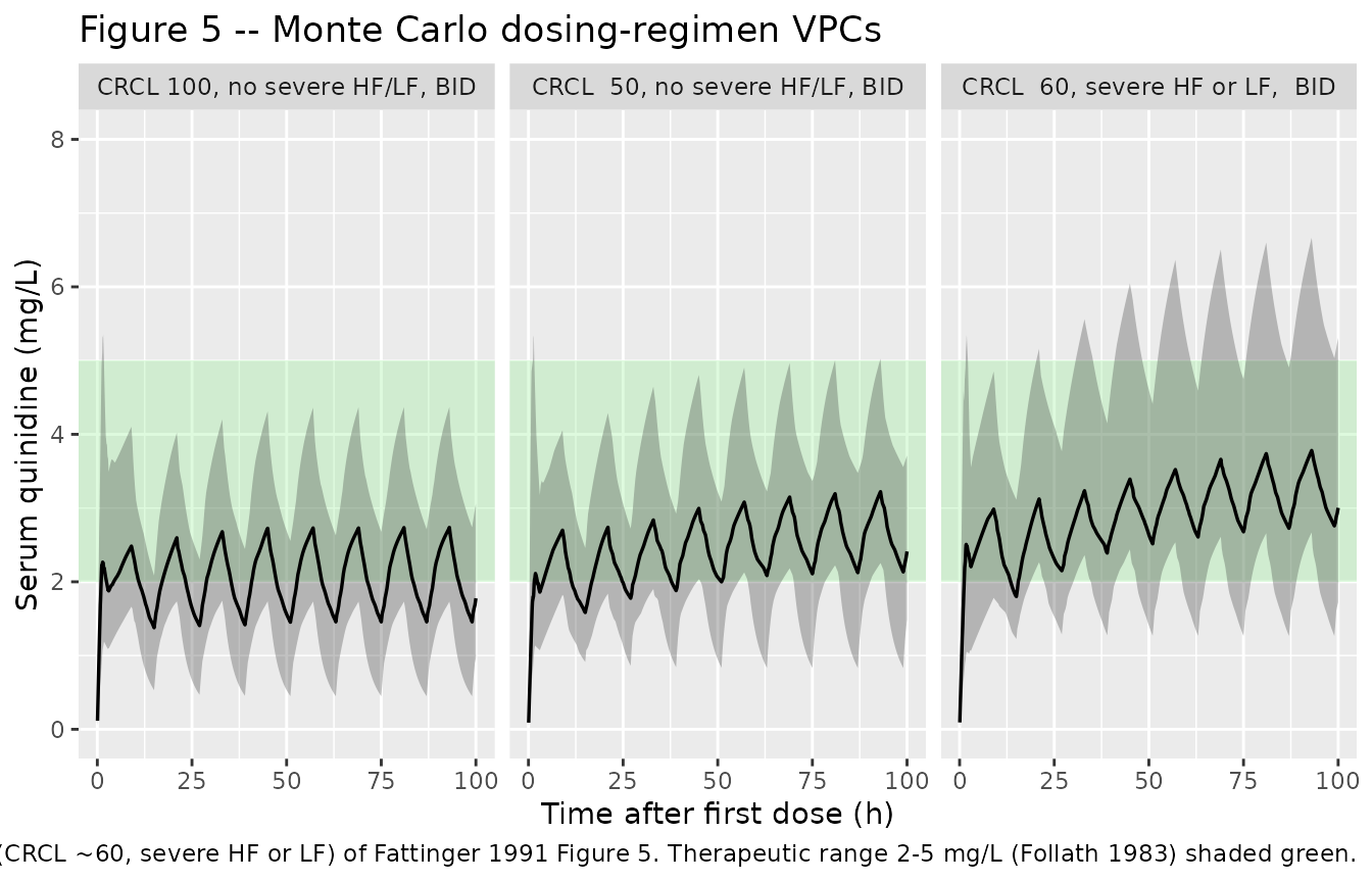
Figure 5 – Monte Carlo dosing-regimen VPCs
# Replicates panels a/c/e of Fattinger 1991 Figure 5 (page 284): VPC of
# serum quinidine concentration vs time across three patient subgroups,
# under the loading-plus-BID regimen described in the abstract item 5.
# The therapeutic range 2-5 mg/L (Follath 1983) is shown as a shaded band.
sim_vpc <- sim |>
  dplyr::filter(!is.na(Cc), Cc >= 0) |>
  dplyr::group_by(time, treatment) |>
  dplyr::summarise(
    Q05 = stats::quantile(Cc, 0.05, na.rm = TRUE),
    Q50 = stats::quantile(Cc, 0.50, na.rm = TRUE),
    Q95 = stats::quantile(Cc, 0.95, na.rm = TRUE),
    .groups = "drop"
  )

ggplot2::ggplot(sim_vpc, ggplot2::aes(time, Q50)) +
  ggplot2::annotate("rect", xmin = -Inf, xmax = Inf, ymin = 2, ymax = 5,
                    fill = "lightgreen", alpha = 0.30) +
  ggplot2::geom_ribbon(ggplot2::aes(ymin = Q05, ymax = Q95), alpha = 0.30) +
  ggplot2::geom_line(linewidth = 0.6) +
  ggplot2::facet_wrap(~ treatment) +
  ggplot2::coord_cartesian(ylim = c(0, 8)) +
  ggplot2::labs(x = "Time after first dose (h)",
                y = "Serum quinidine (mg/L)",
                title = "Figure 5 -- Monte Carlo dosing-regimen VPCs",
                caption = paste0(
                  "Replicates panels a (CRCL >100, no severe HF/LF), c (CRCL ~50, no severe HF/LF), ",
                  "and e (CRCL ~60, severe HF or LF) of Fattinger 1991 Figure 5. ",
                  "Therapeutic range 2-5 mg/L (Follath 1983) shaded green."
                ))
Typical-value profiles (no IIV)
sim_typical |>
  dplyr::filter(!is.na(Cc)) |>
  ggplot2::ggplot(ggplot2::aes(time, Cc, colour = treatment)) +
  ggplot2::annotate("rect", xmin = -Inf, xmax = Inf, ymin = 2, ymax = 5,
                    fill = "lightgreen", alpha = 0.30) +
  ggplot2::geom_line(linewidth = 0.7) +
  ggplot2::coord_cartesian(ylim = c(0, 6)) +
  ggplot2::labs(x = "Time after first dose (h)",
                y = "Serum quinidine (mg/L)",
                colour = "Patient subgroup",
                title = "Typical-value (no IIV) concentration-time profiles")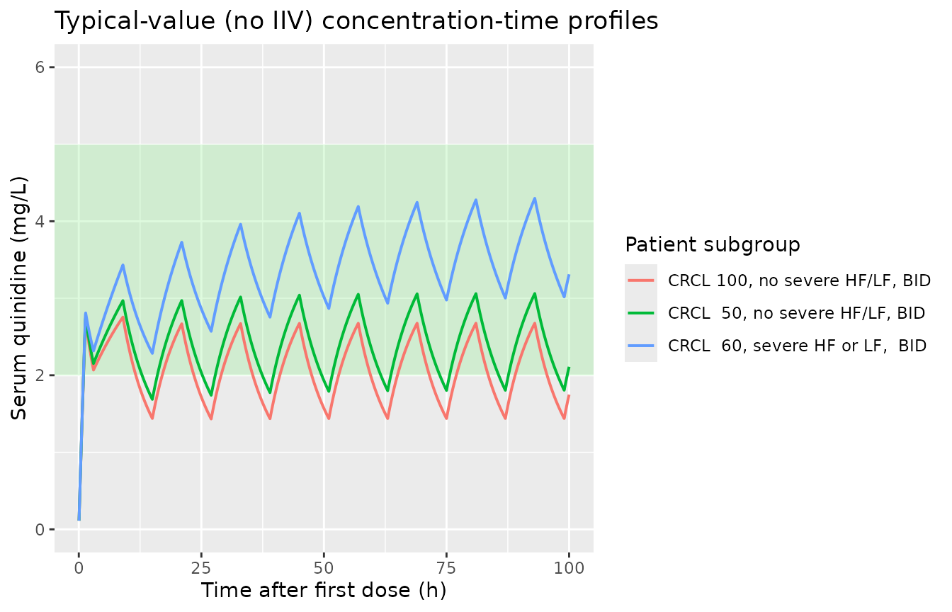
PKNCA validation
Single-dose NCA on a separate simulation lets us cross-check the model’s terminal half-life against the paper’s structural-model value of 10.1 h. We simulate a 600 mg quinidine sulphate single dose in 50 reference-state subjects (CRCL = 100 mL/min, no severe HF/LF) and run PKNCA over a 96 h window to capture the terminal phase.
set.seed(2026)

ids_sd <- seq_len(50)
dose_sd <- data.frame(
  id   = ids_sd,
  time = 0,
  amt  = qs_loading_mg_salt * salt_to_base[["QS"]],
  evid = 1L,
  cmt  = "central",
  rate = -2,
  FORM_QUIN_SR = 0L
)
obs_sd <- expand.grid(id = ids_sd,
                      time = sort(unique(c(seq(0.05, 4, by = 0.1),
                                           seq(4.5, 12, by = 0.5),
                                           seq(13, 96, by = 1)))),
                      KEEP.OUT.ATTRS = FALSE, stringsAsFactors = FALSE)
obs_sd$amt          <- NA_real_
obs_sd$evid         <- 0L
obs_sd$cmt          <- NA_character_
obs_sd$rate         <- NA_real_
obs_sd$FORM_QUIN_SR <- 0L
events_sd <- dplyr::bind_rows(dose_sd, obs_sd)
events_sd$CRCL             <- 100
events_sd$DIS_HF_OR_LF_SEV <- 0L
events_sd$treatment        <- "Single-dose QS reference"

sim_sd <- rxode2::rxSolve(mod, events = events_sd,
                          keep = c("treatment")) |>
  as.data.frame()

sim_nca <- sim_sd |>
  dplyr::filter(!is.na(Cc), Cc > 0) |>
  dplyr::distinct(id, time, .keep_all = TRUE) |>
  dplyr::select(id, time, Cc, treatment) |>
  as.data.frame()

dose_for_nca <- events_sd |>
  dplyr::filter(evid == 1) |>
  dplyr::transmute(id, time, amt, treatment) |>
  as.data.frame()

conc_obj <- PKNCA::PKNCAconc(sim_nca, Cc ~ time | treatment + id,
                             concu = "mg/L", timeu = "h")
dose_obj <- PKNCA::PKNCAdose(dose_for_nca, amt ~ time | treatment + id,
                             doseu = "mg")

intervals_sd <- data.frame(
  start      = 0,
  end        = 96,
  cmax       = TRUE,
  tmax       = TRUE,
  auclast    = TRUE,
  aucinf.obs = TRUE,
  half.life  = TRUE
)

nca_res <- suppressWarnings(
  PKNCA::pk.nca(PKNCA::PKNCAdata(conc_obj, dose_obj, intervals = intervals_sd))
)

nca_tbl <- as.data.frame(nca_res$result)
nca_summary <- nca_tbl |>
  dplyr::group_by(treatment, PPTESTCD) |>
  dplyr::summarise(median = stats::median(PPORRES, na.rm = TRUE),
                   q05    = stats::quantile(PPORRES, 0.05, na.rm = TRUE),
                   q95    = stats::quantile(PPORRES, 0.95, na.rm = TRUE),
                   .groups = "drop")

knitr::kable(nca_summary,
caption = "Single-dose NCA summary (50 virtual reference subjects, 600 mg quinidine sulphate at t=0).")| treatment | PPTESTCD | median | q05 | q95 |
|---|---|---|---|---|
| Single-dose QS reference | adj.r.squared | 0.9999126 | 0.9999017 | 0.9999283 |
| Single-dose QS reference | aucinf.obs | NA | NA | NA |
| Single-dose QS reference | auclast | NA | NA | NA |
| Single-dose QS reference | clast.obs | 0.0024603 | 0.0000506 | 0.0743528 |
| Single-dose QS reference | clast.pred | 0.0024354 | 0.0000499 | 0.0739641 |
| Single-dose QS reference | cmax | 2.4200005 | 0.8910787 | 6.4257447 |
| Single-dose QS reference | half.life | 10.4771610 | 6.5483886 | 28.3071949 |
| Single-dose QS reference | lambda.z | 0.0661617 | 0.0244893 | 0.1058515 |
| Single-dose QS reference | lambda.z.n.points | 90.0000000 | 88.0000000 | 95.5500000 |
| Single-dose QS reference | lambda.z.time.first | 9.5000000 | 6.7250000 | 10.5000000 |
| Single-dose QS reference | lambda.z.time.last | 96.0000000 | 96.0000000 | 96.0000000 |
| Single-dose QS reference | r.squared | 0.9999136 | 0.9999028 | 0.9999291 |
| Single-dose QS reference | span.ratio | 8.1851223 | 3.1090928 | 13.4122973 |
| Single-dose QS reference | tlast | 96.0000000 | 96.0000000 | 96.0000000 |
| Single-dose QS reference | tmax | 1.3500000 | 0.5500000 | 3.0700000 |
Comparison against published structural values
hl_median <- nca_tbl |>
  dplyr::filter(PPTESTCD == "half.life") |>
  dplyr::pull(PPORRES) |>
  stats::median(na.rm = TRUE)

tmax_median <- nca_tbl |>
  dplyr::filter(PPTESTCD == "tmax") |>
  dplyr::pull(PPORRES) |>
  stats::median(na.rm = TRUE)

cl_apparent <- nca_tbl |>
  dplyr::filter(PPTESTCD == "aucinf.obs") |>
  dplyr::pull(PPORRES) |>
  vapply(function(auc) (qs_loading_mg_salt * salt_to_base[["QS"]]) / auc,
         numeric(1)) |>
  stats::median(na.rm = TRUE)

knitr::kable(
  data.frame(
    quantity = c(
      "Terminal half-life (h)",
      "Tmax of QS Cmax (h)",
      "Apparent CL = Dose_base / AUCinf (L/h)"
    ),
    nca_median = c(
      sprintf("%.2f", hl_median),
      sprintf("%.2f", tmax_median),
      sprintf("%.2f", cl_apparent)
    ),
    fattinger_1991 = c(
      "10.1 (page 282)",
      "1.37 (Table 1, t_max,QS)",
      "18.3 (page 282)"
    )
  ),
  caption = "Single-dose NCA median vs Fattinger 1991 structural-model values."
)| quantity | nca_median | fattinger_1991 |
|---|---|---|
| Terminal half-life (h) | 10.48 | 10.1 (page 282) |
| Tmax of QS Cmax (h) | 1.35 | 1.37 (Table 1, t_max,QS) |
| Apparent CL = Dose_base / AUCinf (L/h) | NA | 18.3 (page 282) |
Assumptions and deviations
-
Dose unit convention. Users must supply dose
amounts in mg of quinidine base (apply the Windholz 1983 stoichiometric
factors of 0.829 mg base per mg quinidine sulphate and 0.663 mg base per
mg quinidine bisulphate before passing to the model). The model’s
f(central)term then captures only the formulation-driven relative absorption difference (1 for QS, 1.36 for QBS) and not the stoichiometric salt-to-base conversion. The cohort-building code in this vignette applies the conversion explicitly insidemake_cohortso simulated doses on the input side reflect the salt-form quantities reported by Fattinger 1991. -
Per-dose formulation indicator.
FORM_QUIN_SRis set per dose record in the event table: 0 for quinidine sulphate doses, 1 for quinidine bisulphate doses. The model switchesdur(central)andf(central)at each dose event based on the value present at that event time. The placeholder value on observation rows is ignored. -
Zero-order absorption. Doses are administered to
the central compartment as a zero-order infusion of duration
dur(central), formulation-dependent (exp(ldur_qs + etaldur_qs)for QS,exp(ldur_qbs)for QBS). The IIVetaldur_qsonly affects QS doses; for subjects who receive both formulations the single eta is identifiable from the QS dosing records. -
Pooled severe-HF-or-LF indicator. The paper pools
severe heart failure (n = 2) and severe liver failure (n = 3) into a
single binary covariate (page 282 Results paragraph 4) because the
per-group counts were small and the effect sizes on non-renal CL were
similar. The canonical
DIS_HF_OR_LF_SEVindicator carries this pooled semantic; future users with separate severe-HF and severe-LF subgroups should not split the effect coefficient without further estimation evidence. -
Eta on total CL. The paper’s “interindividual
variability … on clearance” (page 281 / 282) is a single eta in the
NONMEM analysis. We encode this as
etalclacting multiplicatively on the covariate-driven typical-value total CL (renal + non-renal arms), matching the standard NONMEM-stepwise convention. -
Residual error mapping. The paper’s “log-additive
error distribution” (Methods page 281) is conventionally encoded as
proportional residual error in linear space (nlmixr2’s
propSd). -
Validation reproduction. The Figure 5 VPCs are
reproduced for panels a (CRCL >100, no severe HF/LF, BID), c (CRCL
~50, no severe HF/LF, BID), and e (CRCL ~60, severe HF or LF, BID) using
the abstract item 5 regimen (600 mg QS loading dose followed 3 h later
by 500 mg QBS BID). Panels b/d/f (TID regimens) and panel f’s reduced
250 mg TID dose for severe HF/LF are not reproduced here to keep the
example concise; users may modify
qbs_maint_mg_saltandqbs_interval_hin the cohort chunk to explore alternative regimens. - Renal-function range. The paper notes (Discussion page 283) that the model should be used with caution outside the 17 to >100 mL/min CRCL range covered by the cohort. The vignette’s reference-state simulation at CRCL = 100 mL/min and the impaired-cohort simulations at CRCL = 50 and CRCL = 60 mL/min all sit within the original data range.