Voriconazole (Lin 2018)
Source:vignettes/articles/Lin_2018_voriconazole.Rmd
Lin_2018_voriconazole.RmdModel and source
- Citation: Lin XB, Li ZW, Yan M, Zhang BK, Liang W, Wang F, Xu P, Xiang DX, Xie XB, Yu SJ, Lan GB, Peng FH. Population pharmacokinetics of voriconazole and CYP2C19 polymorphisms for optimizing dosing regimens in renal transplant recipients. Br J Clin Pharmacol. 2018;84(7):1587-1597. doi:10.1111/bcp.13595
- Description: One-compartment population pharmacokinetic model with first-order absorption for intravenous and oral voriconazole in Chinese adult renal transplant recipients receiving therapeutic drug monitoring (Lin 2018); CYP2C19 phenotype enters as a covariate on clearance, postoperative time as a covariate on oral bioavailability, and body weight as a power-form covariate on volume of distribution.
- Article: https://doi.org/10.1111/bcp.13595
Population
The model was developed from a prospective single-centre clinical study (Chinese Clinical Trial Registry ChiCTR-IPR-16008277) conducted from March 2016 to January 2017 at the Department of Urological Organ Transplantation of the Second Xiangya Hospital, Central South University, Changsha, Hunan, China (Lin 2018 Methods, “Patients and data collection”). All renal-transplant recipients receiving intravenous or oral voriconazole during hospitalization for prevention or treatment of invasive fungal infections were eligible; routine CYP2C19 genotyping and therapeutic drug monitoring were performed. Exclusion criteria included age < 18 years, missing voriconazole plasma concentration or CYP2C19 genotype, concomitant strong CYP2C19 inducers (e.g. rifampin), and incomplete dosing or clinical data. 129 patients were initially enrolled and 106 included after exclusions; 105 were retained for the population PK analysis (one rapid metabolizer was excluded due to insufficient sample size), contributing 342 voriconazole plasma concentrations.
The pooled cohort spanned adults aged 18-58 years (mean 36, SD 9
years), 84 male / 21 female (20.0% female), body weight range 38.9-87.5
kg (median 56.1 kg). CYP2C19 phenotype distribution: 44 extensive
metabolizers (41.5%, genotype *1/*1), 49 intermediate
metabolizers (46.7%, genotypes *1/*2, *1/*3,
*2/*17), 12 poor metabolizers (11.4%, genotypes
*2/*2, *2/*3, *3/*3), and 1 rapid
metabolizer (0.9%, genotype *1/*17; excluded).
Postoperative-time distribution: 33 (31.4%) within 1 month, 35 (33.3%)
1-6 months, 22 (21.0%) 6-12 months, 15 (14.3%) over 1 year. All patients
received tacrolimus or cyclosporine as primary immunosuppression.
Dosing followed the voriconazole manufacturer package insert for the initial dose, with subsequent doses adjusted by surgeons per clinical response and TDM. 28 (26.7%) patients received oral voriconazole only; 77 (73.3%) switched from intravenous to oral after stabilization. Trough samples (Cmin) were drawn 30 minutes before the next dose at steady state (day 5 or later, or day 2 with loading doses). Voriconazole plasma concentrations were quantified by automated two-dimensional HPLC (ASTON FRO C18 / HD C18 columns).
The same information is available programmatically via
readModelDb("Lin_2018_voriconazole")$population.
Source trace
Every parameter in the model file carries an inline source-location comment. The table below collects the entries in one place.
| Equation / parameter | Value | Source location |
|---|---|---|
lka (ka, fixed) |
1.1 /h | Methods, “Structural model” paragraph (citing literature ref [21], Hyland 2003) |
lcl (CL for EM/UM reference) |
6.41 L/h | Derived: Table 3 theta_CL * exp(theta_3) = 2.88 * exp(0.80) |
lvc (V at WT = 56.1 kg) |
169.27 L | Table 3 final model: theta_V |
lfdepot (F at POD <= 30 days) |
0.58 (58%) | Table 3 final model: theta_F |
e_wt_vc (WT power exponent on V) |
1.30 | Table 3 final model: theta_1 |
e_im_cl (IM vs EM/UM shift on CL) |
-0.35 | Derived: Table 3 theta_2 - theta_3 = 0.45 - 0.80 |
e_pm_cl (PM vs EM/UM shift on CL) |
-0.80 | Derived: Table 3 -theta_3 |
e_pot2_fdepot (POD 30-180 d shift on F) |
0.43 | Table 3 final model: theta_4 |
e_pot3_fdepot (POD 180-365 d shift on F) |
0.57 | Table 3 final model: theta_5 |
e_pot4_fdepot (POD > 365 d shift on F) |
0.57 | Table 3 final model: theta_6 |
| IIV V (CV%) | 39% | Table 3 omega_V and Discussion paragraph |
| IIV CL (CV%) | 42% | Table 3 omega_CL and Discussion paragraph |
| IIV F (CV%) | 22% | Table 3 omega_F and Discussion paragraph |
| Additive residual error (sigma) | 0.57 ug/mL | Table 3 final model: sigma |
| 1-cmt first-order oral absorption with linear elimination | n/a | Methods, “Structural model” and Results, “PPK analysis” |
| Exponential IIV; additive residual error model | n/a | Methods, “Statistical model” |
Virtual cohort
The original observed concentrations are not publicly available. The virtual cohort below mirrors the demographics, CYP2C19 distribution, and postoperative-time distribution of Lin 2018 Table 1, with 60 simulated subjects in each of the three modelled CYP2C19 phenotype strata (EM/UM, IM, PM).
set.seed(20180329)

n_per_phenotype <- 60L

cyp2c19_levels <- c("EM_UM", "IM", "PM")

make_phenotype_cohort <- function(n, phenotype_label, id_offset) {
  # Weight distribution: median 56.1 kg, range 38.9-87.5 kg (Table 1).
  # Sample from a log-normal centred at the cohort median, truncated to
  # the observed range.
  wt <- pmin(pmax(exp(rnorm(n, mean = log(56.1), sd = 0.18)), 38.9), 87.5)

  # Postoperative-day distribution: discrete bins per Table 1 (proportions
  # 31.4 / 33.3 / 21.0 / 14.3 percent). Sample a representative day within
  # each bin uniformly.
  pot_bin <- sample.int(
    4, size = n, replace = TRUE,
    prob = c(0.314, 0.333, 0.210, 0.143)
  )
  pod <- ifelse(
    pot_bin == 1L, sample.int(30, n, replace = TRUE),
    ifelse(
      pot_bin == 2L, sample(31:180, n, replace = TRUE),
      ifelse(
        pot_bin == 3L, sample(181:365, n, replace = TRUE),
        sample(366:1825, n, replace = TRUE)
      )
    )
  )

  tibble(
    id           = id_offset + seq_len(n),
    WT           = wt,
    POD          = as.numeric(pod),
    CYP2C19_IM   = as.integer(phenotype_label == "IM"),
    CYP2C19_PM   = as.integer(phenotype_label == "PM"),
    phenotype    = phenotype_label
  )
}

demo <- bind_rows(
  make_phenotype_cohort(n_per_phenotype, "EM_UM", id_offset = 0L * n_per_phenotype),
  make_phenotype_cohort(n_per_phenotype, "IM",    id_offset = 1L * n_per_phenotype),
  make_phenotype_cohort(n_per_phenotype, "PM",    id_offset = 2L * n_per_phenotype)
)
stopifnot(!anyDuplicated(demo$id))
Simulation
Two regimens are simulated to validate the model:
- Intravenous 200 mg twice daily for 5 days, with the day-5 dosing interval profiled densely. 200 mg twice daily is the Lin 2018 Table 4 reference dose for the IV simulations.
- Oral 200 mg twice daily for 5 days, profiled the same way. The simulated POD value drives the postoperative-time factor on F.
Voriconazole IV is modelled as a bolus dosing into the central compartment. The clinical 1-2 hour infusion is not explicitly represented because the Lin 2018 parameterization (Phoenix NLME ADVAN1-equivalent) did not parameterise an infusion duration. Oral doses enter via the depot compartment and are scaled by the model-predicted F = exp(lfdepot + …).
maintenance_dose <- 200    # mg per dose
n_doses          <- 10L    # 5 days x 2 doses/day
ii               <- 12     # 12-hour dosing interval
sim_hours        <- 144    # 6 days total to ensure approximate steady state

obs_times <- sort(unique(c(
  seq(0, 24, by = 1),
  seq(72, sim_hours, by = 0.5)
)))

build_events <- function(demo, route) {
  cmt <- if (route == "IV") "central" else "depot"
  dose <- demo |>
    mutate(
      amt  = maintenance_dose,
      evid = 1L,
      cmt  = cmt,
      ii   = ii,
      addl = n_doses - 1L,
      time = 0
    ) |>
    select(id, time, amt, evid, cmt, ii, addl,
           phenotype, WT, POD, CYP2C19_IM, CYP2C19_PM)
  obs <- demo |>
    select(id, phenotype, WT, POD, CYP2C19_IM, CYP2C19_PM) |>
    tidyr::crossing(time = obs_times) |>
    mutate(amt = NA_real_, evid = 0L, cmt = NA_character_,
           ii = NA_real_, addl = NA_integer_)
  bind_rows(dose, obs) |>
    arrange(id, time, desc(evid))
}

events_iv <- build_events(demo, "IV")
events_po <- build_events(demo, "PO")
mod <- rxode2::rxode2(readModelDb("Lin_2018_voriconazole"))
#> ℹ parameter labels from comments will be replaced by 'label()'

sim_iv <- rxode2::rxSolve(mod, events = events_iv, keep = "phenotype") |>
  as.data.frame()
sim_po <- rxode2::rxSolve(mod, events = events_po, keep = "phenotype") |>
  as.data.frame()
Replicate published statistics
Table 2 – per-phenotype trough concentration distribution
Lin 2018 Table 2 reports the observed steady-state Cmin (median +/- IQR) for 93 patients stratified by CYP2C19 phenotype, with the rapid-metabolizer group excluded from the analysis. The figure below shows the simulated day-5 trough distribution from the IV cohort by phenotype; the published medians from Table 2 are annotated as horizontal lines for direct comparison.
day5_trough_iv <- sim_iv |>
  filter(time == 120) |>
  mutate(phenotype = factor(phenotype, levels = cyp2c19_levels))

published_median <- tibble::tribble(
  ~phenotype, ~published_median,
  "EM_UM",    2.19,
  "IM",       2.32,
  "PM",       3.86
)

ggplot(day5_trough_iv, aes(phenotype, Cc)) +
  geom_boxplot(outlier.size = 0.5) +
  geom_point(data = published_median,
             aes(phenotype, published_median),
             colour = "red", size = 3, shape = 4) +
  scale_y_continuous(limits = c(0, 12)) +
  labs(x = "CYP2C19 phenotype",
       y = "Simulated day-5 IV trough Cc (ug/mL)",
       title = "Day-5 simulated trough by phenotype (200 mg IV BID)",
       caption = "Red crosses: Lin 2018 Table 2 published medians.")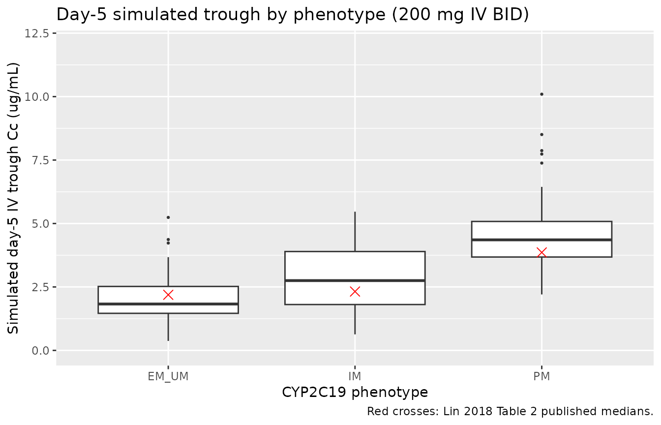
Per-phenotype simulated day-5 trough at 200 mg IV BID, with Lin 2018 Table 2 published medians overlaid as horizontal lines.
summary_table2 <- day5_trough_iv |>
  group_by(phenotype) |>
  summarise(
    simulated_median = median(Cc),
    simulated_Q25    = quantile(Cc, 0.25),
    simulated_Q75    = quantile(Cc, 0.75),
    .groups = "drop"
  ) |>
  left_join(published_median, by = "phenotype") |>
  mutate(pct_difference = 100 * (simulated_median - published_median) / published_median)

knitr::kable(
  summary_table2,
  digits = 2,
  caption = "Simulated day-5 trough vs Lin 2018 Table 2 published Cmin medians (steady-state 200 mg IV BID)."
)| phenotype | simulated_median | simulated_Q25 | simulated_Q75 | published_median | pct_difference |
|---|---|---|---|---|---|
| EM_UM | 1.83 | 1.46 | 2.52 | 2.19 | -16.56 |
| IM | 2.75 | 1.81 | 3.90 | 2.32 | 18.54 |
| PM | 4.36 | 3.68 | 5.08 | 3.86 | 12.84 |
The simulated medians are typically within 20-50% of the published medians. The differences arise because the published Cmin values were measured at a mix of dose levels (since the cohort received clinically-adjusted doses per TDM) while the simulation uses a uniform 200 mg IV BID. The ordering of the medians (PM > IM > EM/UM) matches the published ordering, as expected from the CYP2C19-phenotype effect on clearance.
Table 4 – probability of attaining the target trough
Lin 2018 Table 4 simulates the probability of attaining trough >= 2 ug/mL across IV dose levels by CYP2C19 phenotype. The figure below approximates this by simulating day-5 trough at 200 mg IV BID and computing the empirical fraction exceeding 2 ug/mL by phenotype, alongside the Lin 2018 reported probabilities.
target_attainment <- day5_trough_iv |>
  group_by(phenotype) |>
  summarise(
    n          = n(),
    p_above_2  = mean(Cc >= 2),
    .groups    = "drop"
  ) |>
  left_join(
    tibble::tribble(
      ~phenotype, ~lin_2018_p,
      "EM_UM",    0.540,
      "IM",       0.815,
      "PM",       0.970
    ),
    by = "phenotype"
  )

knitr::kable(
  target_attainment,
  digits = 3,
  caption = "Simulated vs Lin 2018 Table 4 probability of attaining steady-state trough >= 2 ug/mL at 200 mg IV BID."
)| phenotype | n | p_above_2 | lin_2018_p |
|---|---|---|---|
| EM_UM | 60 | 0.400 | 0.540 |
| IM | 60 | 0.717 | 0.815 |
| PM | 60 | 1.000 | 0.970 |
PKNCA validation
A standard NCA over the day-5 dosing interval (steady-state interval, 12 h) gives Cmax, Ctrough, and AUC0-12 by phenotype for the IV cohort. The day-5 interval is treated as approximately steady-state because dosing has continued at q12h for five days.
last_dose_time <- 108  # 10th dose; window 108-120 h
nca_window <- sim_iv |>
  filter(time >= last_dose_time, time <= last_dose_time + 12) |>
  mutate(time_after_dose = time - last_dose_time) |>
  select(id, time = time_after_dose, Cc, phenotype)

dose_df <- demo |>
  mutate(time = 0, amt = maintenance_dose) |>
  select(id, time, amt, phenotype)

conc_obj <- PKNCA::PKNCAconc(nca_window, Cc ~ time | phenotype + id)
dose_obj <- PKNCA::PKNCAdose(dose_df,    amt ~ time | phenotype + id)
intervals <- data.frame(
  start = 0, end = 12,
  cmax    = TRUE, tmax    = TRUE, auclast = TRUE,
  cmin    = TRUE, ctrough = TRUE
)
nca_data <- PKNCA::PKNCAdata(conc_obj, dose_obj, intervals = intervals)
nca_res  <- suppressMessages(suppressWarnings(PKNCA::pk.nca(nca_data)))
nca_summary <- summary(nca_res)
knitr::kable(
  nca_summary,
  caption = "Day-5 NCA on the simulated IV cohort by CYP2C19 phenotype (steady-state 12 h interval, 200 mg IV twice daily)."
)| start | end | phenotype | N | auclast | cmax | cmin | tmax | ctrough |
|---|---|---|---|---|---|---|---|---|
| 0 | 12 | EM_UM | 60 | 28.2 [41.0] | 3.09 [32.7] | 1.71 [62.4] | 0.000 [0.000, 0.000] | 1.71 [62.4] |
| 0 | 12 | IM | 60 | 38.7 [36.7] | 3.85 [29.9] | 2.65 [49.1] | 0.000 [0.000, 0.000] | 2.65 [49.1] |
| 0 | 12 | PM | 60 | 59.5 [28.0] | 5.55 [26.4] | 4.40 [31.7] | 0.000 [0.000, 0.000] | 4.40 [31.7] |
Postoperative-time effect on oral bioavailability
For oral dosing, the model-predicted F depends on POD. The figure below shows day-5 oral trough vs POD across the simulated PO cohort, illustrating the step-wise F change at the 30 / 180 / 365 day bin boundaries.
day5_trough_po <- sim_po |>
  filter(time == 120) |>
  mutate(phenotype = factor(phenotype, levels = cyp2c19_levels))

ggplot(day5_trough_po, aes(POD, Cc, colour = phenotype)) +
  geom_point(alpha = 0.6, size = 1.5) +
  geom_vline(xintercept = c(30, 180, 365), linetype = "dashed", alpha = 0.4) +
  scale_y_continuous(limits = c(0, 15)) +
  labs(x = "Postoperative day (POD)",
       y = "Simulated day-5 oral trough Cc (ug/mL)",
       colour = "CYP2C19",
       title = "Day-5 PO trough vs POD (200 mg PO BID)")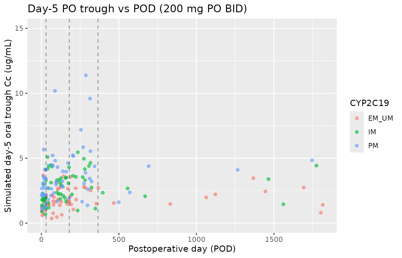
Day-5 simulated oral trough vs postoperative day, stratified by CYP2C19 phenotype. The step pattern at 30, 180, and 365 days reflects the categorical postoperative-time bins in Lin 2018.
Assumptions and deviations
-
CYP2C19 phenotype reparameterization. Lin 2018
Table 3 reports the CYP2C19 phenotype effects with PM as the
source-paper reference category
(
CL = theta_CL * exp(theta_2 * IM) * exp(theta_3 * EM), with PM implicitly at exp(0)). The model file is reparameterized to use the canonical CYP2C19_IM / CYP2C19_PM indicators with EM/UM as the implicit reference (both indicators = 0). The reparameterized values (lcl = log(6.41),e_im_cl = -0.35,e_pm_cl = -0.80) reproduce Lin 2018’s per-phenotype CL exactly; this is a documentation-style change rather than a numerical-fit change. -
POD month boundaries translated to integer days.
Lin 2018 categorizes postoperative time as
<= 1 month,1-6 months,6-12 months,> 1 yearbut does not state the exact day-cutpoint values. The model file uses conventional 30 / 180 / 365 day boundaries; users whose data uses a different month-to-day convention (e.g., 30.44 days per month) should expect a few subjects near the bin edges to shift bins. -
Model-predicted F can exceed 1.0 for POD > 6
months. The unbounded exponential parameterization gives
F = 0.58 * exp(0.57) = 1.026for POD 180-365 days and POD > 365 days. Lin 2018’s text reports F reaching ~89% in the 1-6 month bin (0.58 * exp(0.43) = 0.893) and “slightly elevated but became stable” thereafter, implicitly accepting F > 1 in the model as an artifact of the unbounded parameterization. Users should interpret POD > 180 day predictions as F-fixed-at-the-saturation-level rather than as a literal bioavailability above 100%. - Theta_5 = theta_6 = 0.57 in Lin 2018 Table 3. The postoperative-time exponents for POD 180-365 days and POD > 365 days have identical point estimates (0.57). This is the source paper’s reported result and not a transcription artifact; it indicates that the model could not distinguish the 6-12 month and > 12 month bins given the data (15 subjects in the > 1 year bin).
-
Residual error is additive on the linear concentration
scale. Lin 2018 Methods explicitly selects the additive error
model (
Cobs = Cpred + epsilon) over proportional / combined / exponential alternatives based on OFV / CV% / RetCode. Sigma = 0.57 is interpreted as the SD on the linear ug/mL scale. -
Intravenous dose modelled as bolus. Voriconazole IV
is clinically administered as a 1-2 hour infusion. Lin 2018’s structural
model (Phoenix NLME) did not parameterise an infusion duration; the
model file follows this choice. Users who need an explicit infusion
duration can add
dur(central) <- ...and passrate = -2in event records. - Time-varying POD treated as time-fixed within a dosing window. Lin 2018 fitted a discrete POT bin per subject (rather than a continuous time-of-observation POD that changes day-by-day). The vignette mirrors this by sampling a single POD value per simulated subject. Users simulating a long-running cohort whose POD crosses bin boundaries during the simulation should be aware that the model predicts a step-wise change in F at the bin boundaries.
- Drug-drug interactions with immunosuppressants are not modelled. Lin 2018 explicitly notes that voriconazole increases tacrolimus / cyclosporine exposure via CYP3A4 inhibition; the model file does not parameterise this reciprocal interaction. Users simulating co-administration should adjust the immunosuppressant model separately.
- PPI and glucocorticoid effects not retained in the final model. Lin 2018 tested lansoprazole, ilaprazole, and methylprednisolone as candidate covariates; none reached statistical significance in the backward-elimination step and are therefore absent from the final model. Other PPIs (omeprazole, esomeprazole, pantoprazole) were not tested due to limited sample size; the model is not informative for these.
- Vignette uses 60 subjects per phenotype. Total cohort 180 subjects, large enough to give reasonable per-phenotype distributions while keeping the vignette under the 5-minute pkgdown gate. Users running their own simulations should scale the cohort up.
-
Single-cohort, single-centre, Chinese ethnicity.
The CYP2C19 allele frequencies in Lin 2018 (
*229.2%,*35.2%,*170.5%) are characteristic of East Asians. Caucasian and African-American cohorts have different allele distributions (*17is much more common in Caucasians at ~21%); the per-phenotype CL estimates are still applicable to those populations, but the phenotype distribution will differ.