Ciprofloxacin and desethylene ciprofloxacin (Sima 2022)
Source:vignettes/articles/Sima_2022_ciprofloxacin.Rmd
Sima_2022_ciprofloxacin.RmdModel and source
- Citation: Sima M, Bobek D, Cihlarova P, Rysanek P, Rousarova J, Berousek J, Kuchar M, Vymazal T, Slanar O. Factors Affecting the Metabolic Conversion of Ciprofloxacin and Exposure to Its Main Active Metabolites in Critically Ill Patients: Population Pharmacokinetic Analysis of Desethylene Ciprofloxacin. Pharmaceutics. 2022;14(8):1627. doi:10.3390/pharmaceutics14081627
- Description: One-compartment parent + one-compartment metabolite population PK model for intravenous ciprofloxacin and its active metabolite desethylene ciprofloxacin in 29 critically ill adults (Sima 2022). Both analytes share one volume of distribution Vd and are modelled in MOLAR units (dose in umol, concentrations in umol/L = nmol/mL). Ciprofloxacin is lost by first-order elimination K and by first-order conversion Kpm to desethylene ciprofloxacin, which is eliminated by first-order Km. All covariate effects are exponential in the RAW, UNCENTERED covariate (Monolix log-linear form): age lowers Vd (-0.022 per year) and Km (-0.035 per year), measured creatinine clearance raises Kpm (+0.81 per mL/s), and carriage of at least one CYP1A2 rs762551 variant allele raises Km (+0.6 on the log scale). Proportional residual error on both analytes.
- Article: https://doi.org/10.3390/pharmaceutics14081627 (open access)
Sima 2022 measured ciprofloxacin and three of its active metabolites (desethylene ciprofloxacin, formyl ciprofloxacin and oxociprofloxacin) in critically ill patients. It then built a joint parent-metabolite population PK model for desethylene ciprofloxacin, the metabolite whose metabolic ratio showed the most covariate associations. That joint model is the one packaged here. The other two metabolites are described only by non-compartmental exposure (Table 3) and have no model.
Population
Twenty-nine adult ICU patients (20 men, 9 women) at Motol University Hospital, Prague, were enrolled between February 2019 and June 2020. Each received 400 mg or 600 mg ciprofloxacin every 12 h by intravenous infusion as part of routine care; the regimen was chosen by the treating physician. Table 2 gives the baseline characteristics as median (IQR): age 57 (49-71) years, body weight 90 (70-100) kg, height 175 (168-182) cm, serum creatinine 65 (53-103) umol/L, and measured 24-h urine creatinine clearance 1.29 (0.74-1.91) mL/s. For the CYP1A2 rs762551 polymorphism, 6 patients (20.7%) were wt/wt, 19 (65.5%) wt/v and 4 (13.8%) v/v. Three serum samples were drawn per patient, at 1, 4 and 11.5 h after the end of an infusion, which gives 87 concentrations of each analyte.
The same information is available programmatically via
readModelDb("Sima_2022_ciprofloxacin")()$population.
Source trace
Every ini() value carries an in-file comment pointing to
its source; the table below collects them. All values are from Sima 2022
Table 4. The covariate equations are in the Results section, immediately
above Table 4.
| Equation / parameter | Value | Source location |
|---|---|---|
lvc (Vd_pop) |
log(565.62 L) | Table 4 |
lkel (K_pop) |
log(0.07 1/h) | Table 4 |
lkel_desethylenecip (Km_pop) |
log(3.81 1/h) | Table 4 |
lkmet_desethylenecip (Kpm_pop) |
log(0.017 1/h) | Table 4 |
e_age_vc (beta_Vd_age) |
-0.022 per year | Table 4 |
e_age_kel_desethylenecip (beta_Km_age) |
-0.035 per year | Table 4 |
e_cyp1a2_kel_desethylenecip (beta_Km_CYP1A2_v) |
0.6 | Table 4 |
e_crcl_kmet_desethylenecip (beta_Kpm_CLCR) |
0.81 per mL/s | Table 4 |
etalvc, etalkel,
etalkel_desethylenecip,
etalkmet_desethylenecip
|
0.29^2, 0.24^2, 0.31^2, 0.59^2 | Table 4, ‘Standard deviation of the random effects’ |
propSd, propSd_desethylenecip
|
0.22, 0.25 | Table 4, b1 and b2 |
log(Vd) = log(Vd_pop) + beta_Vd_age * age + eta_Vd |
n/a | Results 3, covariate equations |
log(Km) = log(Km_pop) + beta_Km_age * age + beta_Km_CYP1A2_v * (CYP1A2 = v) + eta_Km |
n/a | Results 3, covariate equations |
log(Kpm) = log(Kpm_pop) + beta_Kpm_CLCR * CLCR + eta_Kpm |
n/a | Results 3, covariate equations |
d/dt(central),
d/dt(central_desethylenecip)
|
n/a | Results 3 and Methods 2.5: one compartment per analyte, first-order elimination of both, unidirectional parent-to-metabolite transfer |
| Molar units | n/a | Methods 2.4 (mass converted to nmol/mL); Figure 1 axis |
Virtual cohort
The observed data are not public. The cohort below draws age and creatinine clearance to match the Table 2 median and IQR, and draws the CYP1A2 carrier status with the observed carrier frequency (23 of 29). Two arms of 200 virtual patients each receive 400 mg or 600 mg every 12 h as a 30-min infusion for five days. The dose is converted to micromoles with the ciprofloxacin molecular weight (331.34 g/mol), because the model is molar.
set.seed(20220804)
rxode2::rxSetSeed(20220804)

mw_cipro <- 331.34 # g/mol
n_per_arm <- 200L
tau <- 12
n_dose <- 10L
t_inf <- 0.5

# Age and creatinine clearance are drawn jointly: the Discussion reports
# that CLCR fell with age (r2 = 0.5774), and the two act in opposite
# directions on the metabolite/parent ratio (age slows Km, CLCR speeds Kpm),
# so drawing them independently would overstate the spread of the ratio.
rho_age_crcl <- -sqrt(0.5774)

make_cohort <- function(n, dose_mg, id_offset = 0L) {
  z_age <- rnorm(n)
  z_crcl <- rho_age_crcl * z_age + sqrt(1 - rho_age_crcl^2) * rnorm(n)
  # Age: normal approximation to median 57, IQR 49-71 (Table 2).
  age <- pmin(pmax(59 + 16 * z_age, 18), 90)
  # Creatinine clearance: log-normal with median 1.29 mL/s and IQR 0.74-1.91,
  # truncated to 0.1-3 mL/s. The CLCR effect on Kpm is an uncentered
  # exponential, exp(0.81 x CLCR), so an untruncated log-normal tail
  # (occasionally > 5 mL/s) would push Kpm far outside the fitted range.
  crcl_ml_s <- pmin(pmax(exp(log(1.29) + log(1.91 / 0.74) / 1.349 * z_crcl), 0.1), 3)
  tibble(
    id = id_offset + seq_len(n),
    treatment = paste(dose_mg, "mg"),
    AGE = age,
    CRCL = crcl_ml_s * 60,
    SNP_CYP1A2_RS762551 = rbinom(n, 1, 23 / 29),
    dose_umol = dose_mg / mw_cipro * 1000
  )
}

subjects <- bind_rows(
  make_cohort(n_per_arm, 400, id_offset = 0L),
  make_cohort(n_per_arm, 600, id_offset = n_per_arm)
)

dose_times <- seq(0, by = tau, length.out = n_dose)
obs_times <- sort(unique(c(
  seq(0, max(dose_times) + tau, by = 0.5),
  # steady-state interval at dose 9 (96-108 h), sampled densely
  96 + c(0.25, 0.75, 1.5, 4.5, 12)
)))

doses <- subjects |>
  tidyr::crossing(time = dose_times) |>
  mutate(evid = 1L, cmt = "central", amt = dose_umol, dur = t_inf, dvid = NA_integer_)
# Observation rows sit on the parent ODE state; `dvid = 1` maps them to the
# first endpoint (Cc). rxode2 still returns both Cc and Cc_desethylenecip as
# columns on every row, and the plots below use those columns.
obs <- subjects |>
  tidyr::crossing(time = obs_times) |>
  mutate(evid = 0L, cmt = "central", amt = NA_real_, dur = NA_real_, dvid = 1L)

events <- bind_rows(doses, obs) |>
  arrange(id, time, desc(evid)) |>
  select(id, time, evid, cmt, amt, dur, dvid, treatment, AGE, CRCL, SNP_CYP1A2_RS762551)
stopifnot(!anyDuplicated(unique(events[, c("id", "time", "evid")])))
Simulation
mod <- readModelDb("Sima_2022_ciprofloxacin")
sim <- rxode2::rxSolve(
  mod,
  events = events,
  keep = c("treatment", "AGE", "CRCL", "SNP_CYP1A2_RS762551"),
  useLinCmt = FALSE
) |>
  as.data.frame()
#> ℹ parameter labels from comments will be replaced by 'label()'
stopifnot(!anyNA(sim$Cc), !anyNA(sim$Cc_desethylenecip))
Typical-patient check against the closed form
Because the two analytes share one volume, the steady-state
metabolite/parent AUC ratio of this model is exactly
Kpm / Km, and the steady-state parent AUC over a dosing
interval is dose / ((K + Kpm) * Vd). The typical patient
below has the cohort medians (57 years, 1.29 mL/s) and carries a CYP1A2
variant allele, like 79% of the cohort.
typ <- data.frame(AGE = 57, CRCL = 1.29 * 60, SNP_CYP1A2_RS762551 = 1)
ini_df <- rxode2::rxode2(mod)$iniDf
#> ℹ parameter labels from comments will be replaced by 'label()'
p <- setNames(ini_df$est, ini_df$name)
vd_typ <- exp(p[["lvc"]] + p[["e_age_vc"]] * typ$AGE)
k_typ <- exp(p[["lkel"]])
km_typ <- exp(p[["lkel_desethylenecip"]] + p[["e_age_kel_desethylenecip"]] * typ$AGE +
  p[["e_cyp1a2_kel_desethylenecip"]] * typ$SNP_CYP1A2_RS762551)
kpm_typ <- exp(p[["lkmet_desethylenecip"]] + p[["e_crcl_kmet_desethylenecip"]] * typ$CRCL / 60)

dose400 <- 400 / mw_cipro * 1000
closed <- c(
  vd = vd_typ, cl_total = (k_typ + kpm_typ) * vd_typ,
  auc_parent = dose400 / ((k_typ + kpm_typ) * vd_typ),
  ratio_pct = 100 * kpm_typ / km_typ
)

ev_typ <- bind_rows(
  data.frame(time = dose_times, evid = 1L, amt = dose400, dur = t_inf, dvid = NA_integer_),
  data.frame(time = seq(96, 108, by = 0.01), evid = 0L, amt = NA_real_, dur = NA_real_, dvid = 1L)
) |>
  mutate(id = 1L, cmt = "central", AGE = typ$AGE, CRCL = typ$CRCL,
         SNP_CYP1A2_RS762551 = typ$SNP_CYP1A2_RS762551) |>
  arrange(time, desc(evid))
sim_typ <- rxode2::rxSolve(rxode2::zeroRe(mod), ev_typ, useLinCmt = FALSE) |>
  as.data.frame()
#> ℹ parameter labels from comments will be replaced by 'label()'
#> ℹ omega/sigma items treated as zero: 'etalvc', 'etalkel', 'etalkel_desethylenecip', 'etalkmet_desethylenecip'
auc_trap <- function(t, y) sum(diff(t) * (head(y, -1) + tail(y, -1)) / 2)
solved <- c(
  auc_parent = auc_trap(sim_typ$time, sim_typ$Cc),
  ratio_pct = 100 * auc_trap(sim_typ$time, sim_typ$Cc_desethylenecip) /
    auc_trap(sim_typ$time, sim_typ$Cc)
)

knitr::kable(
  data.frame(
    Quantity = c(
      "Vd (L)", "Total parent clearance (K + Kpm) x Vd (L/h)",
      "Parent AUC12,ss at 400 mg (umol*h/L)", "Metabolite/parent AUC ratio (%)"
    ),
    `Closed form` = signif(closed, 4),
    `ODE solve` = c(NA, NA, signif(solved, 4)),
    check.names = FALSE
  ),
  caption = "Typical patient: closed form vs. solved ODE (same parameters, so the two agree to numerical precision)."
)| Quantity | Closed form | ODE solve | |
|---|---|---|---|
| vd | Vd (L) | 161.400 | NA |
| cl_total | Total parent clearance (K + Kpm) x Vd (L/h) | 19.100 | NA |
| auc_parent | Parent AUC12,ss at 400 mg (umol*h/L) | 63.210 | 63.210 |
| ratio_pct | Metabolite/parent AUC ratio (%) | 5.119 | 5.119 |
# Same parameters on both sides, so the only difference is the trapezoid on a
# 0.01 h grid and the residual distance from true steady state after 8 doses.
stopifnot(
  abs(solved[["auc_parent"]] / closed[["auc_parent"]] - 1) < 0.01,
  abs(solved[["ratio_pct"]] / closed[["ratio_pct"]] - 1) < 0.01
)
The typical-patient parent AUC12 at 400 mg, about 63.2 umolh/L (=
nmolh/mL), sits on the Table 3 median of 61.89 nmolh/mL. This
is evidence for the structure chosen in the model file: with the
conversion draining the parent, total parent clearance is
(K + Kpm) * Vd. If only K removed parent, the
typical AUC12 would be 106.8 umolh/L at 400 mg, well above the
Table 3 upper quartile of 80.49.
Replicate Figure 1: geometric mean profiles over a dosing interval
Figure 1 of Sima 2022 shows geometric mean serum concentrations at the three sampling times. The maintainers read the points off the figure (plotted at 1.5, 4.5 and 12 h from the start of the infusion; values approximate). The observed points pool the 400 mg and 600 mg patients and samples from different treatment days, so the simulated steady-state interval of each arm brackets them rather than matching one curve.
fig1_obs <- tibble::tribble(
  ~tad, ~analyte, ~gm,
  1.5, "Ciprofloxacin", 8.8,
  4.5, "Ciprofloxacin", 4.3,
  12, "Ciprofloxacin", 2.0,
  1.5, "Desethylene ciprofloxacin", 0.33,
  4.5, "Desethylene ciprofloxacin", 0.26,
  12, "Desethylene ciprofloxacin", 0.15
)

ss <- sim |>
  filter(time >= 96, time <= 108) |>
  mutate(tad = time - 96) |>
  select(id, treatment, tad, Cc, Cc_desethylenecip) |>
  pivot_longer(c(Cc, Cc_desethylenecip), names_to = "analyte", values_to = "conc") |>
  mutate(analyte = ifelse(analyte == "Cc", "Ciprofloxacin", "Desethylene ciprofloxacin"))

ss_gm <- ss |>
  group_by(treatment, analyte, tad) |>
  summarise(gm = exp(mean(log(conc))), .groups = "drop")

ggplot(ss_gm, aes(tad, gm, colour = treatment)) +
  geom_line() +
  geom_point(data = fig1_obs, aes(tad, gm), inherit.aes = FALSE, size = 2.5) +
  facet_wrap(~analyte, scales = "free_y") +
  labs(
    x = "Time from start of infusion (h)",
    y = "Geometric mean concentration (nmol/mL)",
    colour = "Simulated arm",
    caption = "Points: Sima 2022 Figure 1 (digitised). Lines: simulated steady state, dose 9."
  ) +
  theme(legend.position = "bottom")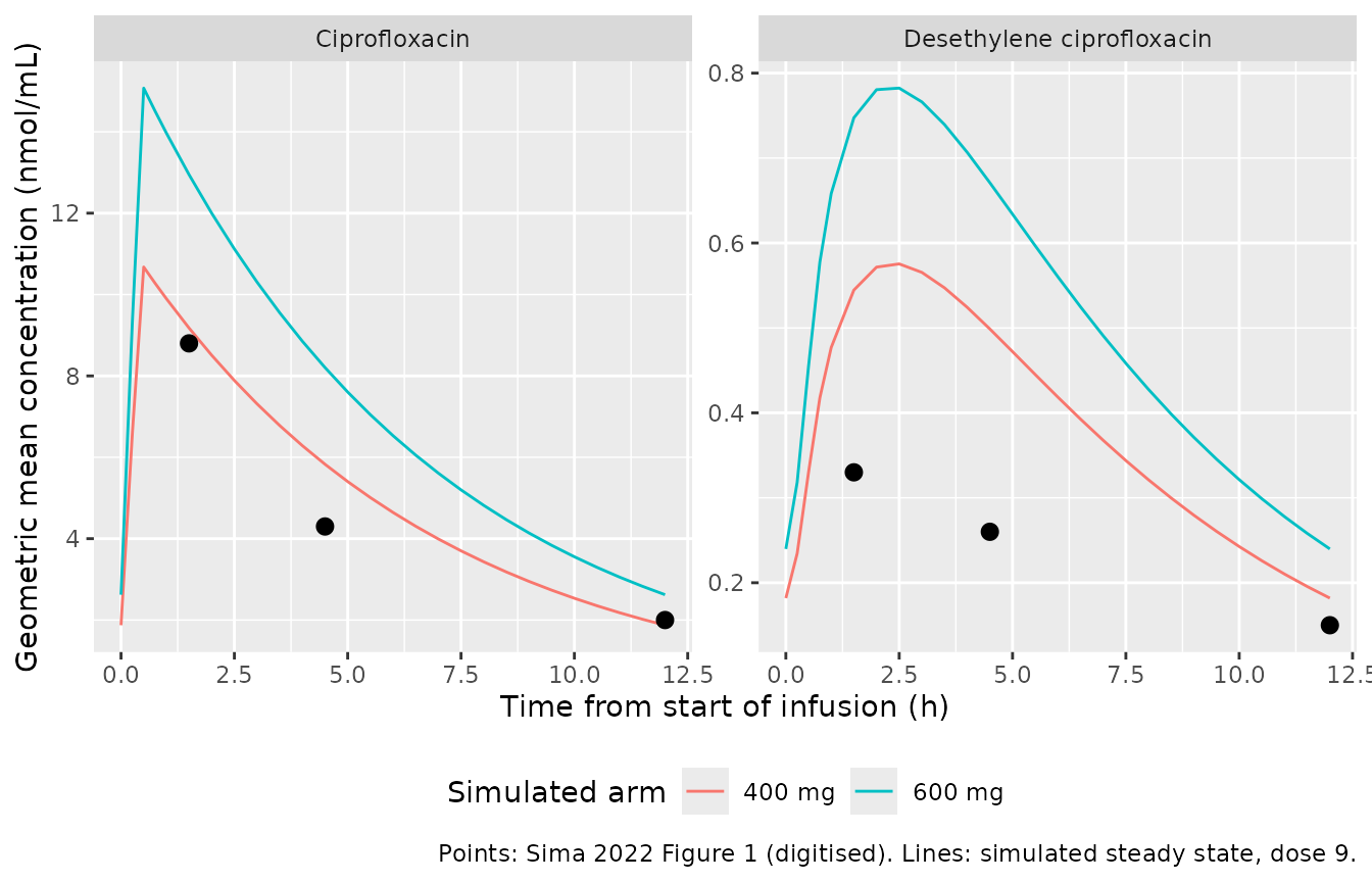
ss_gm |>
  filter(tad %in% c(1.5, 4.5, 12)) |>
  pivot_wider(names_from = treatment, values_from = gm) |>
  left_join(fig1_obs |> rename(published = gm), by = c("analyte", "tad")) |>
  mutate(across(where(is.numeric), ~ signif(.x, 3))) |>
  rename("Analyte" = analyte, "Time (h)" = tad, "Figure 1 (digitised)" = published) |>
knitr::kable(caption = "Geometric mean concentration (nmol/mL) at the Figure 1 sampling times.")| Analyte | Time (h) | 400 mg | 600 mg | Figure 1 (digitised) |
|---|---|---|---|---|
| Ciprofloxacin | 1.5 | 9.180 | 12.900 | 8.80 |
| Ciprofloxacin | 4.5 | 5.830 | 8.200 | 4.30 |
| Ciprofloxacin | 12.0 | 1.870 | 2.620 | 2.00 |
| Desethylene ciprofloxacin | 1.5 | 0.545 | 0.747 | 0.33 |
| Desethylene ciprofloxacin | 4.5 | 0.499 | 0.671 | 0.26 |
| Desethylene ciprofloxacin | 12.0 | 0.182 | 0.240 | 0.15 |
At the Figure 1 sampling times the simulated 400 mg ciprofloxacin geometric means are close to the digitised points at 1.5 and 12 h but higher at 4.5 h, because the simulated decline between 1.5 and 4.5 h is shallower than observed. The observed points fall about two-fold over those 3 h and only two-fold more over the next 7.5 h, which suggests a distribution phase that the published one-compartment model does not describe. The simulated desethylene ciprofloxacin geometric means are about 1.6-fold the digitised values, consistent with the AUC comparison below.
Replicate Figure 4: concentration-time percentiles
Figure 4 is a VPC over the whole sampling period (0 to about 130 h, time since the first dose). The simulated 10th, 50th and 90th percentiles below cover the same window. Figure 4 has a parent median of roughly 6-8 nmol/mL and a desethylene ciprofloxacin median of roughly 0.3-0.4 nmol/mL at the 1-h post-infusion samples. The simulated 400 mg first-dose medians (about 8 and 0.35-0.4 nmol/mL) match those early values. The later simulated intervals sit higher because both analytes accumulate towards steady state, whereas many of the observed samples were taken during the first day of treatment.
sim |>
  select(time, treatment, Cc, Cc_desethylenecip) |>
  pivot_longer(c(Cc, Cc_desethylenecip), names_to = "analyte", values_to = "conc") |>
  mutate(analyte = ifelse(analyte == "Cc", "Ciprofloxacin", "Desethylene ciprofloxacin")) |>
  group_by(treatment, analyte, time) |>
  summarise(
    q10 = quantile(conc, 0.10), q50 = quantile(conc, 0.50), q90 = quantile(conc, 0.90),
    .groups = "drop"
  ) |>
  ggplot(aes(time, q50, colour = treatment, fill = treatment)) +
  geom_ribbon(aes(ymin = q10, ymax = q90), alpha = 0.2, colour = NA) +
  geom_line() +
  facet_wrap(~analyte, scales = "free_y", ncol = 1) +
  labs(
    x = "Time since first dose (h)", y = "Concentration (nmol/mL)",
    colour = "Arm", fill = "Arm",
    caption = "Median and 10th-90th percentiles of individual predictions. Compare Sima 2022 Figure 4."
  ) +
  theme(legend.position = "bottom")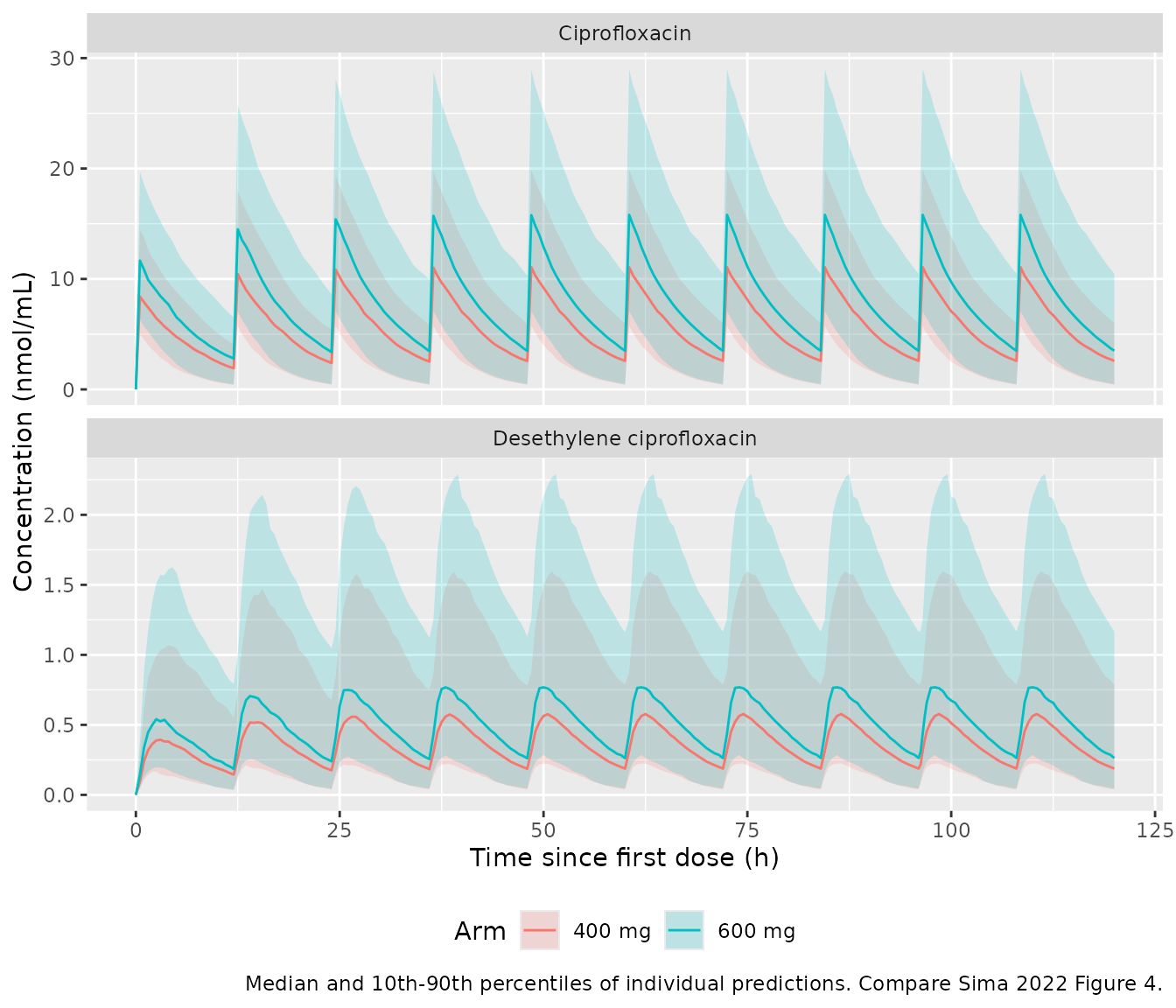
PKNCA validation
PKNCA computes the steady-state AUC over the ninth dosing interval (96-108 h) for each analyte. Table 3 reports AUC12 from the observed samples as median (IQR), pooled over both doses, in nmol*h/mL.
nca_conc <- sim |>
  filter(time >= 96, time <= 108) |>
  select(id, time, treatment, Cc, Cc_desethylenecip) |>
  pivot_longer(c(Cc, Cc_desethylenecip), names_to = "analyte", values_to = "Cc") |>
  mutate(analyte = ifelse(analyte == "Cc", "ciprofloxacin", "desethylene ciprofloxacin")) |>
  filter(!is.na(Cc))

nca_dose <- events |>
  filter(evid == 1) |>
  select(id, time, amt, treatment)

conc_obj <- PKNCA::PKNCAconc(nca_conc, Cc ~ time | treatment + analyte + id)
dose_obj <- PKNCA::PKNCAdose(nca_dose, amt ~ time | treatment + id)
intervals <- data.frame(start = 96, end = 108, auclast = TRUE, cmax = TRUE, cmin = TRUE)
nca_res <- PKNCA::pk.nca(PKNCA::PKNCAdata(conc_obj, dose_obj, intervals = intervals))
nca_tbl <- as.data.frame(nca_res$result)
Comparison against published NCA
published <- tibble::tribble(
  ~treatment, ~analyte, ~auclast,
  "400 mg", "ciprofloxacin", 61.89,
  "600 mg", "ciprofloxacin", 61.89,
  "400 mg", "desethylene ciprofloxacin", 3.30,
  "600 mg", "desethylene ciprofloxacin", 3.30
)

cmp <- nlmixr2lib::ncaComparisonTable(
  simulated = nca_tbl |> filter(PPTESTCD == "auclast"),
  reference = published,
  by = c("treatment", "analyte"),
  units = c(auclast = "nmol*h/mL"),
  tolerance_pct = 20
)
knitr::kable(cmp, caption = "Simulated median steady-state AUC12 vs. the pooled Table 3 median.")| NCA parameter | treatment | analyte | Reference | Simulated | % diff |
|---|---|---|---|---|---|
| AUClast (nmol*h/mL) | 400 mg | ciprofloxacin | 61.9 | 71.1 | +14.9% |
| AUClast (nmol*h/mL) | 400 mg | desethylene ciprofloxacin | 3.3 | 4.78 | +45.0%* |
| AUClast (nmol*h/mL) | 600 mg | ciprofloxacin | 61.9 | 96.7 | +56.3%* |
| AUClast (nmol*h/mL) | 600 mg | desethylene ciprofloxacin | 3.3 | 6.24 | +89.2%* |
For ciprofloxacin, the 400 mg arm lands close to the pooled Table 3 median and the 600 mg arm is about 1.5-fold higher, as a linear model must be. The paper does not report how many patients received each dose or on which treatment day they were sampled. The observed AUC12 values pool both doses and include samples taken before steady state, which lowers them, so the parent comparison is only approximate.
Desethylene ciprofloxacin is over-predicted: the simulated median AUC12 is roughly 1.4-1.5-fold the Table 3 median in the 400 mg arm, and more in the 600 mg arm. Most of this comes through the metabolite/parent ratio below, whose simulated median runs about 25% above Table 3. The parameters were not adjusted to close the gap; see the next section and Assumptions and deviations.
Metabolite/parent ratio (dose-independent)
The molar metabolite/parent AUC12 ratio does not depend on dose, so it is the cleanest comparison with Table 3 (median 5.86%, IQR 4.09-9.87%).
ratio <- nca_tbl |>
  filter(PPTESTCD == "auclast") |>
  select(id, treatment, analyte, PPORRES) |>
  pivot_wider(names_from = analyte, values_from = PPORRES) |>
  mutate(ratio_pct = 100 * `desethylene ciprofloxacin` / ciprofloxacin)

ratio_summary <- ratio |>
  summarise(
    median = median(ratio_pct),
    q25 = quantile(ratio_pct, 0.25),
    q75 = quantile(ratio_pct, 0.75)
  )

bind_rows(
  tibble(Source = "Sima 2022 Table 3", median = 5.86, q25 = 4.09, q75 = 9.87),
  ratio_summary |> mutate(Source = "Simulated (both arms)")
) |>
  mutate(across(where(is.numeric), ~ round(.x, 2))) |>
  rename("Median (%)" = median, "Q1 (%)" = q25, "Q3 (%)" = q75) |>
knitr::kable(caption = "Desethylene ciprofloxacin / ciprofloxacin AUC12 ratio.")| Source | Median (%) | Q1 (%) | Q3 (%) |
|---|---|---|---|
| Sima 2022 Table 3 | 5.86 | 4.09 | 9.87 |
| Simulated (both arms) | 7.30 | 4.37 | 12.27 |
# Centre and robust quartiles only (never the extremes). A mis-transcribed
# Kpm, Km or covariate coefficient moves the ratio two-fold or more. The
# simulated median sits about 25% above Table 3 (7.3% vs 5.86% on the
# authoring run), so the bound is set at 1.6-fold to leave room for
# cohort-to-cohort variation of the median (about +/-12% at 400 subjects).
stopifnot(
  abs(log(ratio_summary$median / 5.86)) < log(1.6),
  ratio_summary$q25 > 2, ratio_summary$q75 < 20
)
Assumptions and deviations
Known deviation: desethylene ciprofloxacin exposure. With the published parameters, the simulated cohort’s median metabolite/parent AUC12 ratio is about 7% against 5.86% in Table 3. The simulated metabolite AUC12 and the Figure 1 geometric means run about 1.5-fold above the published values. For the typical patient (57 years, 1.29 mL/s, variant carrier) the model gives a ratio of 5.1%, close to the published median. The cohort median sits higher because of the uncentered age and creatinine-clearance terms and the large Kpm variability (omega 0.59) applied to a virtual cohort whose covariate joint distribution approximates, but cannot reproduce, the 29 actual patients. The paper’s AUC12 values are also non-compartmental, computed from three samples with the linear trapezoidal rule, not model predictions. The values were kept as published.
Units. Sima 2022 converted all concentrations to nmol/mL before analysis (Methods 2.4), and the Figure 1 and Figure 4 axes are on that scale. The model is therefore molar: dose in umol of ciprofloxacin and concentrations in umol/L (= nmol/mL). Convert a mass dose with the ciprofloxacin molecular weight, 331.34 g/mol (400 mg = 1207 umol). The transfer to desethylene ciprofloxacin is molar, so no molecular-weight correction applies to it. Multiply by 331.34 (ciprofloxacin) or 305.30 (desethylene ciprofloxacin) to obtain ng/mL from nmol/mL.
The conversion drains the parent. The paper describes “the unidirectional transformation from the parent drug to the metabolite” in Monolix, whose transfer macro removes the amount from the source compartment. Total ciprofloxacin loss is therefore
(K + Kpm) * central. The typical-patient check above supports this reading: the draining structure reproduces the Table 3 parent AUC12 and the non-draining one does not.Shared volume. The paper parameterises the model with one volume of distribution (Vd) and no separate metabolite volume, so both analytes use
vc.Uncentered covariates. The covariate equations are exponential in raw age and raw creatinine clearance (in mL/s), so
lvc,lkel_desethylenecipandlkmet_desethylenecipare values at age 0 or CLCR 0. They are not typical-patient values; the typical patient’s values are computed above.Creatinine clearance in mL/min. The
CRCLcolumn is in mL/min and the model divides it by 60 because the published coefficient is per mL/s. The paper’s CLCR is a measured 24-h urine creatinine clearance and is not BSA-normalized.Which allele is the CYP1A2 variant. The paper defines the covariate as “at least one variant allele” at rs762551 but does not say whether the variant is the A or the C allele. The covariate column
SNP_CYP1A2_RS762551keeps the paper’s wt/v labelling. It is not interchangeable withSNP_CYP1A2_RS762551_C_CARRIER, because an A-carrier and a C-carrier indicator disagree for every homozygote.Infusion duration. The paper does not state the infusion duration. The maintainers used 30 min, because Figure 1 plots the samples taken 1, 4 and 11.5 h after the end of the infusion at 1.5, 4.5 and 12 h.
Dose split and sampling day. The numbers of patients on 400 mg and 600 mg, and the treatment day on which each patient was sampled, are not reported. The vignette simulates the two doses as separate arms at steady state.
Virtual covariates. Age is drawn from a normal distribution approximating the Table 2 median and IQR, truncated to 18-90 years, and creatinine clearance from a log-normal distribution matching its median and IQR, truncated to 0.1-3 mL/s (6-180 mL/min). The two are drawn with a correlation of -0.76, the square root of the r2 = 0.5774 the Discussion reports for the decline of CLCR with age (applied here on the log-CLCR scale, an approximation). The truncation matters because the creatinine-clearance effect on Kpm is an uncentered exponential: at 5 mL/s it multiplies Kpm by 57, far outside anything the 29-patient cohort (IQR 0.74-1.91 mL/s) could have informed. Users simulating patients with very high measured creatinine clearance should keep this in mind.
Figure values. The Figure 1 geometric means were digitised by the maintainers and are approximate.
No correction notice for Sima 2022 was found in Europe PMC as of 2026-10-09.