Model and source
- Citation: Smit C, Wasmann RE, Goulooze SC, Wiezer MJ, van Dongen EPA, Mouton JW, Bruggemann RJM, Knibbe CAJ. Population pharmacokinetics of vancomycin in obesity: Finding the optimal dose for (morbidly) obese individuals. Br J Clin Pharmacol. 2020;86(2):303-317. doi:10.1111/bcp.14144.
- Description: Three-compartment population PK model for intravenous vancomycin in morbidly obese adults undergoing bariatric surgery and nonobese healthy volunteers (Smit 2020). Clearance scales with total body weight by an estimated power exponent; the first peripheral volume (V2) scales linearly with total body weight; central (V1) and first peripheral volume share a linear age effect centred on 36.5 years. Between-subject variability on clearance is estimated separately for the obese and nonobese cohorts, selected by DIS_OBESE_MORBID.
- Article: Br J Clin Pharmacol 2020;86(2):303-317 (open access, PMC7015748)
Population
Smit 2020 enrolled 20 morbidly obese adults scheduled for laparoscopic sleeve gastrectomy or gastric bypass (median weight 139.0 kg, range 110.6-234.6; median BMI 45.5 kg/m^2, range 40.8-65.7; median age 38.0 years, range 23-54) and 8 nonobese healthy volunteers (median weight 69.5 kg, range 60.0-84.7; median BMI 21.2 kg/m^2; median age 25.5 years, range 20-55) at St. Antonius Hospital, Nieuwegein, The Netherlands (Table 1). Renal impairment (eGFR < 60 mL/min/1.73 m^2) was an exclusion criterion; median measured 24-h creatinine clearance was 141.4 mL/min in the obese and 117.9 mL/min in the nonobese group. The sex distribution is not reported.
Obese patients received a single 12.5 mg/kg infusion of vancomycin (maximum 2500 mg) during or immediately after surgery; nonobese volunteers received 1000 mg. All infusions ran at 10 mg/min. 326 plasma samples were taken over 48 h (11-13 per subject), and the 24 samples (7%) below the 1.5 mg/L limit of detection were handled with the M3 method.
The same information is available programmatically via
readModelDb("Smit_2020_vancomycin")()$population.
Source trace
Every ini() value carries an in-file comment pointing to
the source. All values are from the final-model column of Smit 2020
Table 2.
| Equation / parameter | Value | Source location |
|---|---|---|
lcl (CL at 70 kg) |
log(5.72) L/h | Table 2, CL70kg |
e_wt_cl |
0.535 | Table 2, theta1 in CL70kg x (TBW/70)^theta1 |
lvc (V1 at 36.5 y) |
log(16.7) L | Table 2, V1_36.5yr |
e_age_vc_vp |
0.0136 /year | Table 2, theta2 (same estimate listed under both V1 and V2) |
lq (Q V1-V2) |
log(15.8) L/h | Table 2 |
lvp (V2 at 70 kg, 36.5 y) |
log(6.98) L | Table 2, V2_70kg;36.5yr |
lq2 (Q V1-V3) |
log(5.21) L/h | Table 2 |
lvp2 (V3) |
log(19.5) L | Table 2 |
etalcl (nonobese) |
fixed(0.002784) | Table 2, IIV CL nonobese 5.28% FIX; footnote b |
etalcl_obese |
0.05920 | Table 2, IIV CL obese 24.7%; footnote b |
etalvc |
0.18664 | Table 2, IIV V1 45.3%; footnote b |
propSd |
0.0392 | Table 2, proportional error; footnote c (‘shown as sigma’) |
addSd |
1.07 mg/L | Table 2, additive error |
cl = CL70kg * (WT/70)^theta1 |
n/a | Table 2 row header |
vc = V1_36.5yr * (1 + theta2 * (AGE - 36.5)) |
n/a | Table 2 row header |
vp = V2 * (WT/70) * (1 + theta2 * (AGE - 36.5)) |
n/a | Table 2 row header |
| Three-compartment, first-order elimination | n/a | Results 3.1 |
| Combined additive + proportional error | n/a | Results 3.1 |
IIV was reported as CV% computed as sqrt(exp(omega^2) - 1) (Table 2
footnote b), so each variance is
omega^2 = log(1 + CV^2).
mod <- readModelDb("Smit_2020_vancomycin")
mod_typical <- rxode2::zeroRe(mod)
#> ℹ parameter labels from comments will be replaced by 'label()'
#> Warning: some etas defaulted to non-mu referenced, possible parsing error: etalcl_obese
#> as a work-around try putting the mu-referenced expression on a simple line
#> Warning: some etas defaulted to non-mu referenced, possible parsing error: etalcl_obese
#> as a work-around try putting the mu-referenced expression on a simple line
Single-dose simulation of the study design
A virtual cohort of 200 obese and 200 nonobese subjects reproduces the study’s dosing: 12.5 mg/kg (maximum 2500 mg) or 1000 mg, infused at 10 mg/min. Obese weights are drawn log-normally around the Table 1 median (139 kg) and truncated to the observed range; nonobese weights around 69.5 kg. Ages are drawn uniformly across each group’s Table 1 range.
set.seed(2020)
n_arm <- 200

make_cohort <- function(n, obese, id_offset) {
  if (obese) {
    wt <- pmin(pmax(exp(rnorm(n, log(139), 0.2)), 110.6), 234.6)
    age <- runif(n, 23, 54)
    dose <- pmin(12.5 * wt, 2500)
  } else {
    wt <- pmin(pmax(exp(rnorm(n, log(69.5), 0.1)), 60), 84.7)
    age <- runif(n, 20, 55)
    dose <- rep(1000, n)
  }
  subj <- tibble(
    id = id_offset + seq_len(n),
    WT = wt,
    AGE = age,
    DIS_OBESE_MORBID = as.integer(obese),
    group = if (obese) "Morbidly obese" else "Nonobese",
    amt = dose,
    rate = 600 # 10 mg/min = 600 mg/h
  )
  obs_times <- sort(unique(c(seq(0, 12, by = 0.25), seq(13, 96, by = 1))))
  doses <- subj |> mutate(time = 0, evid = 1L, cmt = "central")
  obs <- subj |>
    select(id, WT, AGE, DIS_OBESE_MORBID, group) |>
    tidyr::crossing(time = obs_times) |>
    mutate(evid = 0L, amt = 0, rate = 0, cmt = "central")
  bind_rows(doses, obs) |> arrange(id, time, desc(evid))
}

events <- bind_rows(
  make_cohort(n_arm, obese = TRUE, id_offset = 0L),
  make_cohort(n_arm, obese = FALSE, id_offset = n_arm)
)
stopifnot(!anyDuplicated(unique(events[, c("id", "time", "evid")])))
sim <- rxode2::rxSolve(
  mod,
  events = events,
  keep = c("group", "WT", "DIS_OBESE_MORBID")
) |>
  as.data.frame()
#> ℹ parameter labels from comments will be replaced by 'label()'
#> Warning: some etas defaulted to non-mu referenced, possible parsing error: etalcl_obese
#> as a work-around try putting the mu-referenced expression on a simple line
Concentration-time profiles (cf. Figure 1)
sim |>
  filter(time <= 48) |>
  group_by(group, time) |>
  summarise(
    Q025 = quantile(sim, 0.025, na.rm = TRUE),
    Q50 = quantile(sim, 0.50, na.rm = TRUE),
    Q975 = quantile(sim, 0.975, na.rm = TRUE),
    .groups = "drop"
  ) |>
  ggplot(aes(time, Q50)) +
  geom_ribbon(aes(ymin = pmax(Q025, 0.1), ymax = Q975), alpha = 0.25) +
  geom_line() +
  geom_hline(yintercept = 1.5, linetype = "dotted", colour = "grey40") +
  facet_wrap(~group) +
  scale_y_log10() +
  labs(
    x = "Time after start of infusion (h)",
    y = "Vancomycin concentration (mg/L)",
    title = "Simulated median and 95% interval, single dose",
    caption = paste(
      "Compare with the pcVPCs in Figure 1 of Smit 2020 (observed data are not",
      "public). Dotted line: 1.5 mg/L limit of detection."
    )
  )
#> Warning in transformation$transform(x): NaNs produced
#> Warning in scale_y_log10(): log-10 transformation introduced infinite values.
#> Warning in transformation$transform(x): NaNs produced
#> Warning in scale_y_log10(): log-10 transformation introduced infinite values.
#> Warning: Removed 2 rows containing missing values or values outside the scale range
#> (`geom_line()`).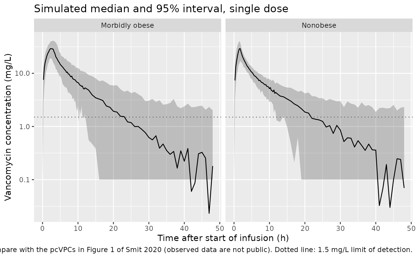
PKNCA validation
The paper reports no NCA table, so the NCA is checked against the model itself. For each subject, the single-dose AUC0-inf must equal the dose divided by that subject’s individual clearance. Both sides use the same drawn parameters, so the only differences are the trapezoidal error and the lambda-z extrapolation.
sim_nca <- sim |>
  filter(!is.na(Cc)) |>
  select(id, time, Cc, group)
sim_nca <- bind_rows(
  sim_nca,
  sim_nca |> distinct(id, group) |> mutate(time = 0, Cc = 0)
) |>
  distinct(id, group, time, .keep_all = TRUE) |>
  arrange(id, group, time)

dose_df <- events |>
  filter(evid == 1) |>
  mutate(duration = amt / rate) |>
  select(id, time, amt, duration, group)

conc_obj <- PKNCA::PKNCAconc(sim_nca, Cc ~ time | group + id)
dose_obj <- PKNCA::PKNCAdose(
  dose_df, amt ~ time | group + id,
  route = "intravascular", duration = "duration"
)
intervals <- data.frame(
  start = 0, end = Inf,
  cmax = TRUE, tmax = TRUE, aucinf.obs = TRUE, half.life = TRUE
)
nca_res <- PKNCA::pk.nca(PKNCA::PKNCAdata(conc_obj, dose_obj, intervals = intervals))

nca_wide <- as.data.frame(nca_res) |>
  filter(PPTESTCD %in% c("cmax", "aucinf.obs", "half.life")) |>
  select(id, group, PPTESTCD, PPORRES) |>
  tidyr::pivot_wider(names_from = PPTESTCD, values_from = PPORRES)

indiv_cl <- sim |>
  group_by(id) |>
  summarise(cl = first(cl), .groups = "drop")

chk <- nca_wide |>
  left_join(dose_df |> select(id, amt), by = "id") |>
  left_join(indiv_cl, by = "id") |>
  mutate(auc_expected = amt / cl, pct_diff = 100 * (aucinf.obs - auc_expected) / auc_expected)

chk |>
  group_by(group) |>
  summarise(
    "Median Cmax (mg/L)" = median(cmax),
    "Median AUC0-inf (mg*h/L)" = median(aucinf.obs),
    "Median t1/2 (h)" = median(half.life),
    "Median AUC % diff vs dose/CL" = median(pct_diff),
    "90th pct |% diff|" = quantile(abs(pct_diff), 0.9),
    .groups = "drop"
  ) |>
  rename("Group" = group) |>
knitr::kable(digits = 2, caption = "PKNCA single-dose summary and AUC0-inf check against dose / individual CL.")| Group | Median Cmax (mg/L) | Median AUC0-inf (mg*h/L) | Median t1/2 (h) | Median AUC % diff vs dose/CL | 90th pct |% diff| |
|---|---|---|---|---|---|
| Morbidly obese | 32.53 | 206.82 | 5.68 | -0.12 | 0.22 |
| Nonobese | 28.82 | 174.65 | 6.75 | -0.16 | 0.31 |
Dosing simulations
The paper’s dosing simulations (Methods 2.7) used obese individuals with a uniform weight distribution between 90 and 230 kg receiving continuous infusions, with day-3 AUC24h (48-72 h) compared against 400 mgh/L (PTA) and 700 mgh/L (PTOX). The simulation age distribution is not stated; the reference age of 36.5 years is used here, and Figure A4 of the paper reports no clinically significant age effect.
Figure 3C: 35 mg/kg/day continuous infusion, maximum 5500 mg/day
Because only clearance determines the day-3 AUC once the infusion is
near steady state, and CL is log-normal in the obese group with variance
etalcl_obese, PTA and PTOX follow in closed form from the
typical-value day-3 AUC. The typical-value AUC comes from a
deterministic solve.
wt_grid <- sort(c(seq(90, 230, by = 10), 155))
ci_events <- function(wt, id, mg_per_kg = 35, cap = 5500, ld = 0) {
  rate_ci <- min(mg_per_kg * wt, cap) / 24
  t_ci <- if (ld > 0) 2 else 0
  obs <- tibble(time = seq(0, 72, by = 0.1), evid = 0L, amt = 0, rate = 0)
  ci <- tibble(time = t_ci, evid = 1L, amt = rate_ci * (72 - t_ci), rate = rate_ci)
  doses <- if (ld > 0) bind_rows(tibble(time = 0, evid = 1L, amt = ld, rate = 600), ci) else ci
  bind_rows(doses, obs) |>
    mutate(id = id, WT = wt, AGE = 36.5, DIS_OBESE_MORBID = 1L, cmt = "central") |>
    arrange(time, desc(evid))
}
auc_window <- function(time, conc, from, to) {
  keep <- time >= from & time <= to
  t <- time[keep]
  y <- conc[keep]
  sum(diff(t) * (head(y, -1) + tail(y, -1)) / 2)
}

ev_typ <- bind_rows(lapply(seq_along(wt_grid), function(i) ci_events(wt_grid[i], i)))
sim_typ <- rxode2::rxSolve(mod_typical, events = ev_typ, keep = "WT") |> as.data.frame()
#> ℹ omega/sigma items treated as zero: 'etalcl', 'etalcl_obese', 'etalvc'
#> Warning: multi-subject simulation without without 'omega'

omega_cl <- sqrt(0.05920) # etalcl_obese
fig3 <- sim_typ |>
  group_by(id, WT) |>
  summarise(auc_d3 = auc_window(time, Cc, 48, 72), cl = first(cl), .groups = "drop") |>
  mutate(
    dose = pmin(35 * WT, 5500),
    auc_ss = dose / cl,
    pct_of_ss = 100 * auc_d3 / auc_ss,
    PTA = pnorm(log(auc_d3 / 400) / omega_cl),
    PTOX = 1 - pnorm(log(700 / auc_d3) / omega_cl),
    P_below_900 = pnorm(log(900 / auc_d3) / omega_cl)
  )

fig3 |>
  select(WT, dose, auc_d3, pct_of_ss, PTA, PTOX, P_below_900) |>
  rename(
    "Weight (kg)" = WT, "Daily dose (mg)" = dose,
    "Typical day-3 AUC24h (mg*h/L)" = auc_d3, "Day-3 AUC as % of steady state" = pct_of_ss,
    "PTA (AUC > 400)" = PTA, "PTOX (AUC > 700)" = PTOX, "P(AUC < 900)" = P_below_900
  ) |>
knitr::kable(digits = c(0, 0, 0, 1, 3, 3, 3), caption = "35 mg/kg/day (max 5500 mg/day) continuous infusion, day 3.")| Weight (kg) | Daily dose (mg) | Typical day-3 AUC24h (mg*h/L) | Day-3 AUC as % of steady state | PTA (AUC > 400) | PTOX (AUC > 700) | P(AUC < 900) |
|---|---|---|---|---|---|---|
| 90 | 3150 | 481 | 99.9 | 0.775 | 0.061 | 0.995 |
| 100 | 3500 | 505 | 99.9 | 0.831 | 0.090 | 0.991 |
| 110 | 3850 | 528 | 99.9 | 0.873 | 0.123 | 0.986 |
| 120 | 4200 | 550 | 99.9 | 0.905 | 0.161 | 0.979 |
| 130 | 4550 | 571 | 99.9 | 0.928 | 0.201 | 0.969 |
| 140 | 4900 | 591 | 99.9 | 0.946 | 0.243 | 0.958 |
| 150 | 5250 | 610 | 99.9 | 0.959 | 0.286 | 0.945 |
| 155 | 5425 | 620 | 99.9 | 0.964 | 0.308 | 0.938 |
| 160 | 5500 | 618 | 99.9 | 0.963 | 0.303 | 0.939 |
| 170 | 5500 | 598 | 99.9 | 0.951 | 0.258 | 0.954 |
| 180 | 5500 | 580 | 100.0 | 0.937 | 0.219 | 0.965 |
| 190 | 5500 | 563 | 100.0 | 0.920 | 0.186 | 0.973 |
| 200 | 5500 | 548 | 100.0 | 0.902 | 0.157 | 0.979 |
| 210 | 5500 | 534 | 100.0 | 0.882 | 0.133 | 0.984 |
| 220 | 5500 | 521 | 100.0 | 0.861 | 0.112 | 0.988 |
| 230 | 5500 | 509 | 100.0 | 0.838 | 0.095 | 0.990 |
The paper states for this regimen (Results 3.4) that PTA was below 90% but still above 80% for individuals below 110 kg and above 210 kg, that PTOX peaked around 150-160 kg, and that 94% of individuals at 150-160 kg had an AUC24h below 900 mg*h/L. The model reproduces all four claims. The one exception is the 90 kg edge of the simulated weight range, where the closed-form PTA is 78%. The paper summarises PTA per weight category; averaged over the 90, 100 and 110 kg grid points the closed-form PTA is 83%.
# These are deterministic (a typical-value solve plus the log-normal CDF),
# so the bounds do not depend on the random-number stream.
pta_in <- function(w) fig3$PTA[fig3$WT %in% w]
stopifnot(
  # 100-110 kg and 210-230 kg: PTA below 90% but above 80%
  all(pta_in(c(100, 110, 210, 220, 230)) > 0.80),
  all(pta_in(c(100, 110, 210, 220, 230)) < 0.90),
  # 130-200 kg: at least 90%
  all(pta_in(seq(130, 200, by = 10)) >= 0.90),
  # PTOX peaks where the 5500 mg/day cap starts to bind (about 157 kg)
  fig3$WT[which.max(fig3$PTOX)] %in% c(150, 155, 160),
  # about 94% of individuals at 150-160 kg below 900 mg*h/L
  all(abs(fig3$P_below_900[fig3$WT %in% c(150, 155, 160)] - 0.94) < 0.02),
  # the day-3 AUC is essentially at steady state, so Figure 3 does not
  # depend on whether a loading dose was given
  all(abs(fig3$pct_of_ss - 100) < 1)
)
A stochastic cohort (200 per weight band) shows the same picture with Monte Carlo noise.
set.seed(3)
bands <- c(100, 130, 160, 190, 220)
n_band <- 200
ev_mc <- bind_rows(lapply(seq_along(bands), function(b) {
  wts <- runif(n_band, bands[b] - 15, bands[b] + 15)
  bind_rows(lapply(seq_len(n_band), function(j) {
    ci_events(wts[j], (b - 1) * n_band + j) |>
      filter(evid == 1 | time >= 48) |>
      mutate(band = paste0(bands[b] - 15, "-", bands[b] + 15, " kg"))
  }))
}))
sim_mc <- rxode2::rxSolve(mod, events = ev_mc, keep = c("band", "WT")) |>
  as.data.frame() |>
  mutate(band = factor(band, levels = paste0(bands - 15, "-", bands + 15, " kg")))
mc <- sim_mc |>
  group_by(id, band) |>
  summarise(auc_d3 = auc_window(time, Cc, 48, 72), .groups = "drop")

mc |>
  group_by(band) |>
  summarise(
    "Mean AUC24h" = mean(auc_d3),
    "2.5th pct" = quantile(auc_d3, 0.025),
    "97.5th pct" = quantile(auc_d3, 0.975),
    "PTA" = mean(auc_d3 > 400),
    "PTOX" = mean(auc_d3 > 700),
    .groups = "drop"
  ) |>
  rename("Weight band" = band) |>
knitr::kable(digits = 2, caption = "Stochastic replicate of Figure 3C (n = 200 per band).")| Weight band | Mean AUC24h | 2.5th pct | 97.5th pct | PTA | PTOX |
|---|---|---|---|---|---|
| 85-115 kg | 513.68 | 297.82 | 820.56 | 0.81 | 0.07 |
| 115-145 kg | 583.16 | 376.79 | 910.45 | 0.94 | 0.20 |
| 145-175 kg | 618.05 | 367.64 | 944.71 | 0.96 | 0.28 |
| 175-205 kg | 572.90 | 340.43 | 869.81 | 0.92 | 0.18 |
| 205-235 kg | 535.37 | 320.11 | 827.83 | 0.88 | 0.09 |
ggplot(mc, aes(band, auc_d3)) +
  geom_boxplot() +
  geom_hline(yintercept = c(400, 700), linetype = "dashed", colour = "grey50") +
  labs(
    x = "Weight band", y = "Day-3 AUC24h (mg*h/L)",
    caption = "Replicates the left panel of Figure 3C of Smit 2020 (35 mg/kg/day, maximum 5500 mg/day)."
  )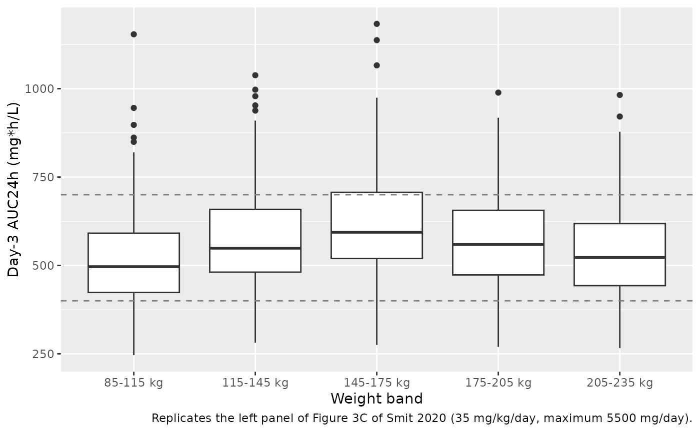
Figure 4: loading dose before a continuous infusion
The paper recommends a 1500 mg loading dose (10 mg/min) followed 2 h after its start by the 35 mg/kg/day continuous infusion, reporting a day-1/day-3 AUC24h ratio close to 1 at every weight. The typical-value ratios are:
lds <- c(500, 1000, 1500, 2000, 2500)
ev_ld <- bind_rows(lapply(seq_along(lds), function(k) {
  bind_rows(lapply(seq_along(wt_grid), function(i) {
    ci_events(wt_grid[i], (k - 1) * length(wt_grid) + i, ld = lds[k]) |> mutate(ld = lds[k])
  }))
}))
sim_ld <- rxode2::rxSolve(mod_typical, events = ev_ld, keep = c("WT", "ld")) |> as.data.frame()
#> ℹ omega/sigma items treated as zero: 'etalcl', 'etalcl_obese', 'etalvc'
#> Warning: multi-subject simulation without without 'omega'
ratios <- sim_ld |>
  group_by(id, WT, ld) |>
  summarise(ratio = auc_window(time, Cc, 0, 24) / auc_window(time, Cc, 48, 72), .groups = "drop")

ggplot(ratios, aes(WT, ratio, colour = factor(ld))) +
  geom_line() +
  geom_hline(yintercept = 1, linetype = "dashed", colour = "grey50") +
  labs(
    x = "Weight (kg)", y = "AUC24h day 1 / AUC24h day 3", colour = "Loading dose (mg)",
    caption = "Typical-value replicate of Figure 4 of Smit 2020."
  )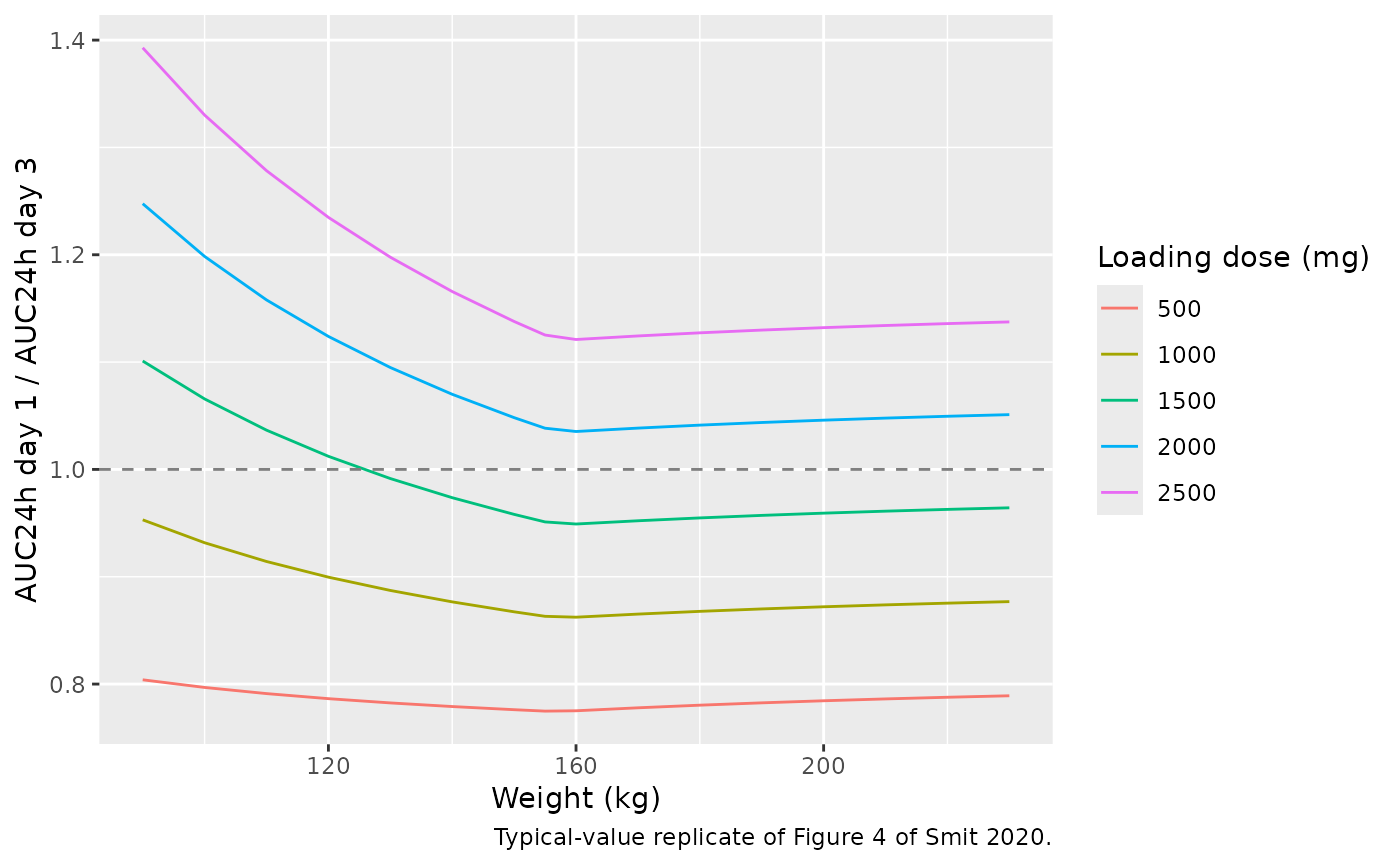
With 1500 mg, the typical ratio stays between 0.95 and 1.1 across 90-230 kg.
Figure 5: trough concentration versus AUC24h, twice-daily dosing
For 35 mg/kg/day (maximum 5500 mg/day) given as two infusions per day at 10 mg/min, the paper reports that the trough concentrations matching the 400-700 mg*h/L AUC24h window span 5.7-14.6 mg/L. The paper samples the trough 0.5 h before the second dose of day 3.
set.seed(5)
n_bid <- 200
wts_bid <- runif(n_bid, 90, 230)
ev_bid <- bind_rows(lapply(seq_len(n_bid), function(j) {
  dose <- min(35 * wts_bid[j], 5500) / 2
  bind_rows(
    tibble(time = seq(0, 60, by = 12), evid = 1L, amt = dose, rate = 600),
    tibble(time = c(seq(48, 72, by = 0.25), 59.5), evid = 0L, amt = 0, rate = 0)
  ) |>
    distinct(time, evid, .keep_all = TRUE) |>
    mutate(id = j, WT = wts_bid[j], AGE = 36.5, DIS_OBESE_MORBID = 1L, cmt = "central") |>
    arrange(time, desc(evid))
}))
sim_bid <- rxode2::rxSolve(mod, events = ev_bid, keep = "WT") |> as.data.frame()
bid <- sim_bid |>
  group_by(id, WT) |>
  summarise(
    auc_d3 = auc_window(time, Cc, 48, 72),
    trough = Cc[which.min(abs(time - 59.5))],
    .groups = "drop"
  )
in_window <- bid |> filter(auc_d3 >= 400, auc_d3 <= 700)
trough_range <- quantile(in_window$trough, c(0.025, 0.975))

ggplot(bid, aes(trough, auc_d3)) +
  geom_point(alpha = 0.5) +
  geom_smooth(method = "lm", formula = y ~ x, se = FALSE, colour = "black") +
  geom_hline(yintercept = c(400, 700), linetype = "dashed") +
  geom_vline(xintercept = trough_range, colour = "red") +
  labs(
    x = "Day-3 trough concentration (mg/L)", y = "Day-3 AUC24h (mg*h/L)",
    caption = "Replicates Figure 5A of Smit 2020 (n = 200 here, 10 000 in the paper)."
  )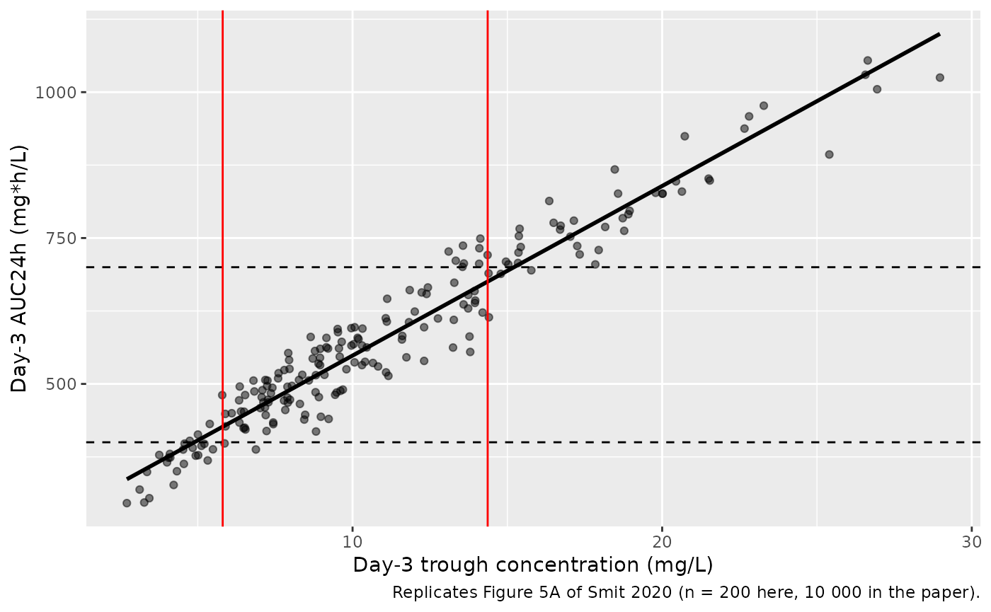
The 2.5th-97.5th percentiles of the trough among simulated subjects in the AUC window are 5.8-14.4 mg/L, against 5.7-14.6 mg/L in the paper.
Figure A4: age
ages <- c(20, 30, 40, 50)
ev_age <- bind_rows(lapply(seq_along(ages), function(i) {
  ci_events(130, i, ld = 1500) |> filter(time <= 24 | evid == 1) |> mutate(AGE = ages[i])
}))
rxode2::rxSolve(mod_typical, events = ev_age, keep = "AGE") |>
  as.data.frame() |>
  ggplot(aes(time, Cc, colour = factor(AGE))) +
  geom_line() +
  labs(
    x = "Time (h)", y = "Vancomycin concentration (mg/L)", colour = "Age (years)",
    caption = paste(
      "Replicates Figure A4 of Smit 2020: 130 kg, 1500 mg loading dose then",
      "35 mg/kg/day continuous infusion from 2 h."
    )
  )
#> ℹ omega/sigma items treated as zero: 'etalcl', 'etalcl_obese', 'etalvc'
#> Warning: multi-subject simulation without without 'omega'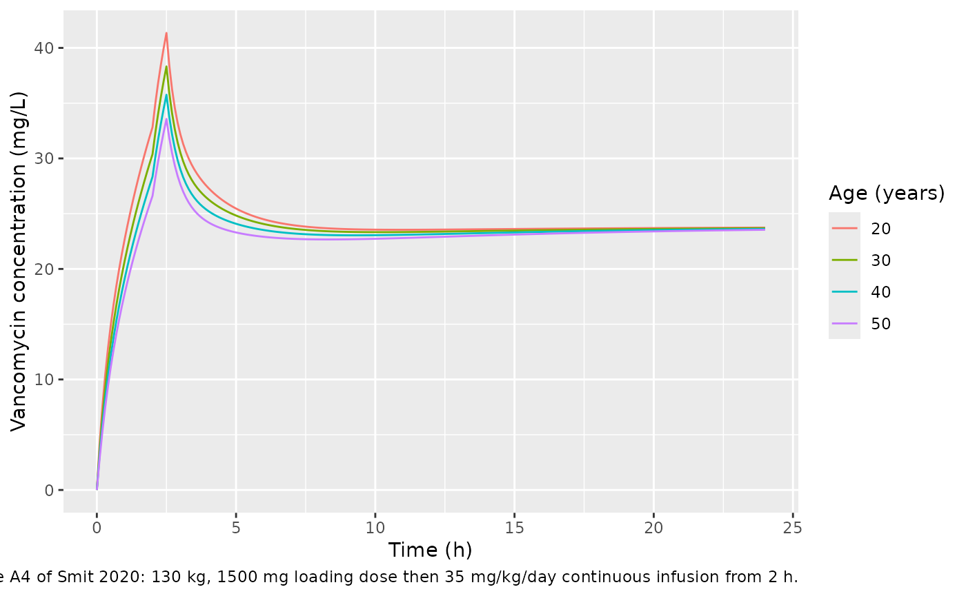
Assumptions and deviations
-
Cohort-specific CL variability. Table 2 gives
separate IIV on CL for the nonobese (5.28%, fixed) and obese (24.7%)
groups with a single typical value. The model draws both etas and
selects one with
DIS_OBESE_MORBID. Each group’s variance is therefore exact, butetalcl_obeseis not mu-referenced. This affects re-estimation efficiency, not simulation; the load-time note about non-mu-referenced etas is expected. -
Shared age slope. Table 2 lists theta2 = 0.0136
under both V1 and V2 with identical precision, so it is encoded as one
parameter (
e_age_vc_vp) used in both equations. - Residual error scale. Table 2 footnote c states the proportional error is shown as sigma (a standard deviation). The additive error is taken as an SD in mg/L by the same convention.
- Simulation cohorts. The paper’s dosing simulations used 10 000 individuals and did not state the age distribution. Here the closed-form PTA/PTOX use the reference age of 36.5 years, and the stochastic replicates use 200 subjects per band. The single-dose cohort weights are log-normal around the Table 1 medians, since individual weights are not published.
- Figure 3 without a loading dose. The Methods do not say whether the Figure 3 regimens included a loading dose. The day-3 AUC is simulated without one; the typical day-3 AUC is already within a few percent of steady state (table above), so a loading dose barely changes it.
- PTOX level. The closed-form PTOX at 150-160 kg is about 30%. The paper’s Discussion describes PTOX as below 20% “for most individuals” across the whole 90-230 kg range, and gives no per-weight value to compare against. The 94% below 900 mg*h/L at 150-160 kg, which it does give, is reproduced.
- BLQ handling. The M3 method was used for estimation only and has no effect on the model structure.
- No erratum or correction notice linked to this article (PMID
- was found in Europe PMC as of 2026-09-25.