Avatrombopag (Liu 2025)
Source:vignettes/articles/Liu_2025_avatrombopag.Rmd
Liu_2025_avatrombopag.RmdModel and source
- Citation: Liu X, Chen L, Ju G, Li C, Liu B, Fei Y, Wang X, Gao Y, He Q, Zhu X, Ouyang D. (2025). Investigation of the ABCB1 Gene Polymorphism and Food Effects on the Avatrombopag Pharmacokinetics in Chinese Individuals: A Population Pharmacokinetic/ Pharmacodynamic Analysis. Pharmaceuticals 18(6):903. doi:10.3390/ph18060903
- Description: Population PK model for avatrombopag in 92 healthy Chinese adults given a single 20 mg oral dose under fasting or high-fat-fed conditions in a two-sequence, four-period replicate bioequivalence trial. One-compartment disposition with first-order elimination preceded by a nine-transit-compartment absorption chain (dose -> depot -> transit1 .. transit9, transfer rate ktr = 9 / MTT) followed by first-order absorption (ka) from transit9 into the central compartment. A food-by-genotype co-effect acts on the absorption fraction Fa (relative bioavailability): Fa = 1 + COV1 * FED_HIGHFAT + COV2 * (1 - ABCB1_C1236T_HET) + COV3 * FED_HIGHFAT * (1 - ABCB1_C1236T_HET), so the reference Fa = 1 is a fasting ABCB1 (C1236T) TC heterozygote. Between-subject variability is estimated on CL/F, Vd/F, ka and MTT; inter-occasion variability is estimated on ka across the four study periods. The source paper additionally simulated platelet counts by linking this PK model to a previously published chronic-liver-disease platelet-count PK/PD life-span model (Nomoto 2018, J Clin Pharmacol 58:1629-1638); no PD parameter of that model is reported in Liu 2025, so only the PK layer is implemented here.
- Article (open access): https://doi.org/10.3390/ph18060903
Avatrombopag is an orally active, second-generation thrombopoietin receptor agonist (TPO-RA) approved for thrombocytopenia in chronic liver disease and in chronic immune thrombocytopenia. It is a BCS Class II compound whose absorption is solubility-limited, so its exposure is unusually sensitive to food, and it is a substrate of both CYP2C9 and the P-glycoprotein efflux transporter encoded by ABCB1. Liu 2025 asks whether that combination of food and pharmacogenetic sensitivity is large enough to warrant dose individualisation in Chinese patients.
What this paper contains, and what is packaged here
Liu 2025 has three analytical layers:
- A non-compartmental analysis of a four-period bioequivalence trial, comparing exposure across food conditions, sexes, and CYP2C9 / ABCB1 genotypes (Tables 1, 2, and S1-S7).
- An original population PK model built in NONMEM 7.5
from all 5923 avatrombopag concentrations. Its structure and every
parameter estimate are reported in Table 3. This is the model
packaged as
Liu_2025_avatrombopagand validated below. - A PK/PD simulation of platelet-count trajectories.
The PD layer is not this paper’s model: Methods 4.5 states that
“a previously published PD model developed in chronic liver disease
(CLD) patients [10] was adopted and linked to our PK model”, with a 32%
slope reduction applied for East Asians. Reference [10] is Nomoto, Ferry
and Hussein (2018), J Clin Pharmacol 58:1629-1638,
doi:10.1002/jcph.1267. Liu 2025 reports no PD parameter of that model at all – no baseline, no lifespan, no slope, no turnover rate, no residual error – so the PD layer cannot be source-traced from any available source and is deliberately not implemented here. See “Assumptions and deviations” for the details, including which of the paper’s own PD numbers can be back-solved and which cannot.
Population
Liu 2025 pooled 92 healthy Chinese volunteers enrolled at the Clinical Trials Unit of Hunan Province People’s Hospital (Changsha, Hunan) into a single-centre, open-label, two-sequence, four-period replicate bioequivalence trial with a 14-day washout between periods. Each subject received a single 20 mg avatrombopag tablet with 200 mL of water in each period. Forty-seven subjects were dosed after an overnight fast and 45 were dosed roughly 30 min after an FDA-standard high-fat, high-calorie breakfast (800-1000 kcal, of which 500-600 kcal from fat); the two arms are disjoint subject groups with separately tabulated demographics (Table 1).
pop <- rxode2::rxode(readModelDb("Liu_2025_avatrombopag"))$population
#> ℹ parameter labels from comments will be replaced by 'label()'
#> Warning: some etas defaulted to non-mu referenced, possible parsing error: etaiov_ka_1, etaiov_ka_2, etaiov_ka_3, etaiov_ka_4
#> as a work-around try putting the mu-referenced expression on a simple line
tibble::tibble(Field = names(pop), Value = vapply(pop, paste, character(1), collapse = "; ")) |>
knitr::kable(caption = "Population metadata carried in the model file (Liu 2025 Table 1, Results 2.1 and Methods 4.1-4.4).")| Field | Value |
|---|---|
| species | human |
| n_subjects | 92 |
| n_studies | 1 |
| n_pk_observations | 5923 |
| age_range | 18-45 years |
| age_median | 28 years |
| weight_range | mean 63.22 +/- 7.88 kg (fasting arm) and 60.95 +/- 6.32 kg (fed arm) |
| sex_female_pct | 9.8 |
| race_ethnicity | Chinese (single-centre Chinese cohort; no further ethnic breakdown reported) |
| disease_state | healthy volunteers |
| dose_range | single 20 mg oral avatrombopag tablet with 200 mL water, repeated over four periods separated by a 14-day washout; 47 subjects dosed under an overnight fast and 45 dosed about 30 min after a high-fat, high-calorie meal |
| regions | China (Clinical Trials Unit of Hunan Province People’s Hospital, Changsha, Hunan) |
| genotypes | CYP2C9: 90% 1/1 normal metabolizer, 10% 1/3 intermediate metabolizer, no 3/3. ABCB1 (C1236T): 14% CC, 51% TC, 35% TT. ABCB1 (C3435T): 40% CC, 47% TC, 13% TT. ABCB1 (G2677T/A): 20% GG, 67% heterozygous, 13% homozygous variant. All variants were in Hardy-Weinberg equilibrium (Results 2.1, 2.2.2 and Table 1). |
| notes | Open-label, single-centre, two-sequence, four-period replicate bioequivalence trial (IRB approval [2023]-32.1, Hunan Province People’s Hospital). Sampling at predose and 1, 2, 3, 4, 5, 6, 7, 8, 9, 10, 11, 12, 16, 24, 48, 72 and 96 h post dose; plasma avatrombopag by UPLC-MS/MS with an AVA-D8 internal standard, linear range 1.000-400.000 ng/mL. Estimation in NONMEM 7.5 with FOCE-I; stepwise covariate modelling (forward p < 0.05, backward p < 0.01); evaluated by GOF plots, VPC and non-parametric bootstrap (Table 3). Baseline demographics are Liu 2025 Table 1. |
Plasma avatrombopag was measured by UPLC-MS/MS against an AVA-D8 internal standard over a 1.000-400.000 ng/mL calibration range, with samples at predose and 1, 2, 3, 4, 5, 6, 7, 8, 9, 10, 11, 12, 16, 24, 48, 72 and 96 h after each dose.
Source trace
Every structural element and every ini() value traces to
Liu 2025 Table 3 or to the Methods text. Table 3’s covariate rows are
labelled only COV1-COV3; their meaning comes
from the table footnote, reproduced verbatim in the last three rows
below.
| Element | Value | Source location |
|---|---|---|
| One-compartment disposition, first-order elimination | structure | Results 2.3: ‘A one-compartment model with nine transit compartments, along with first-order absorption and elimination, was selected as the final model.’ |
| Nine transit absorption compartments, ktr = 9 / MTT | structure | Results 2.3 (same sentence); ktr convention per
nlmixr2lib lktr = n_transit / MTT |
| Exponential IIV, combined proportional + additive residual error | structure | Methods 4.4: ‘IIV was modeled using an exponential approach, while residual variability was tested using proportional, additive, and combined error models’ |
| lcl = log(7.85) | CL/F = 7.85 L/h (RSE 14%) | Table 3, row ‘CL/F (L/h)’ |
| lvc = log(199) | Vd/F = 199 L (RSE 13%) | Table 3, row ‘Vd/F (L)’ |
| lka = log(0.582) | ka = 0.582 /h (RSE 13%) | Table 3, row ‘ka (/h)’ |
| lmtt = log(1.33) | MTT = 1.33 h (RSE 5%) | Table 3, row ‘MTT (h)’ |
| lfdepot = fixed(log(1)) | reference Fa = 1 | Table 3 footnote: ‘Fa = 1 x (1 + COV1 x FOOD + COV2 x ABCB1 + COV3 x FOOD x ABCB1)’ |
| e_fed_highfat_fdepot = -0.0653 | COV1 (RSE 111%) | Table 3, row ‘COV1’; footnote ‘the effect of fed state and TC genotype on Fa’ |
| e_abcb1hom_fdepot = -0.272 | COV2 (RSE 15%) | Table 3, row ‘COV2’; footnote ‘the effect of fast state and non-TC genotype on Fa’ |
| e_fed_abcb1hom_fdepot = 0.177 | COV3 (RSE 56%) | Table 3, row ‘COV3’; footnote ‘the effect of fed state and non-TC genotype on Fa’ |
| etalcl ~ 0.182 | BSV on CL/F (RSE 35%); 44.7% CV | Table 3, ‘Between-subject variability’ block, row ‘CL/F’ |
| etalvc ~ 0.159 | BSV on Vd/F (RSE 32%); 41.6% CV | Table 3, ‘Between-subject variability’ block, row ‘Vd/F’ |
| etalka ~ 0.504 | BSV on ka (RSE 35%); 81.6% CV | Table 3, ‘Between-subject variability’ block, row ‘KA’ |
| etalmtt ~ 0.131 | BSV on MTT (RSE 23%); 37.5% CV | Table 3, ‘Between-subject variability’ block, row ‘MTT’ |
| etaiov_ka_1..4 ~ 0.913 | IOV on ka (RSE 12%); 122% CV | Table 3, ‘Between-subject variability’ block, row ‘OCC [KA]’ |
| propSd = 0.239 | proportional residual error 23.90% (RSE 4%) | Table 3, ‘Residual unexplained variability’ block, row ‘sigma prop (%)’ |
| addSd = 1.18 | additive residual error 1.18 ng/mL (RSE 3%) | Table 3, ‘Residual unexplained variability’ block, row ‘sigma add (ng/mL)’ |
| FOOD = 1 fed / 0 fasting | covariate coding | Table 3 footnote: ‘If in the fed state, FOOD is 1; fasting state is 0.’ |
| ABCB1 = 1 homozygote / 0 heterozygote | covariate coding | Table 3 footnote: ‘If the genotype is heterozygote, ABCB1 is 0; homozygote is 1.’ |
| Four occasions per subject | OCC = 1..4 | Methods 4.2: ‘This open-label, crossover study consisted of four periods with two sequences, separated by a 14-day washout.’ |
The absorption-fraction covariate model
Table 3’s footnote is the only place the covariate model appears, and
its two indicator conventions are both non-obvious:
FOOD = 1 marks the fed state, and
ABCB1 = 1 marks a homozygote (either CC wild-type
or TT variant) while ABCB1 = 0 marks the TC heterozygote.
The canonical nlmixr2lib column ABCB1_C1236T_HET runs the
other way (1 = heterozygote), so the model file writes
(1 - ABCB1_C1236T_HET) wherever the paper writes
ABCB1. The four strata evaluate to:
| Stratum | FED_HIGHFAT | ABCB1_C1236T_HET | Fa |
|---|---|---|---|
| Fasting, ABCB1 (C1236T) TC | 0 | 1 | 1.0000 |
| Fed, TC | 1 | 1 | 0.9347 |
| Fasting, non-TC (CC or TT) | 0 | 0 | 0.7280 |
| Fed, non-TC | 1 | 0 | 0.8397 |
The reference stratum (Fa = 1) is therefore a fasting TC
heterozygote, and the paper’s headline finding – “a 1.37-fold
increase in Cmax and AUC … the comparison between the TC and non-TC
under fasting state” (Results 2.4) – is exactly
1 / 0.728 = 1.374.
Virtual cohort
The single-dose cohort replicates the trial as designed: 47 fasting and 45 fed subjects, each contributing four 20 mg occasions, with ABCB1 (C1236T) genotypes assigned at the per-arm counts of Table 1 (fasting 7 CC / 28 TC / 12 TT; fed 6 CC / 19 TC / 20 TT). Both arms are well under the 200-per-arm cap.
set.seed(20250616)

mod <- rxode2::rxode(readModelDb("Liu_2025_avatrombopag"))
#> ℹ parameter labels from comments will be replaced by 'label()'
#> Warning: some etas defaulted to non-mu referenced, possible parsing error: etaiov_ka_1, etaiov_ka_2, etaiov_ka_3, etaiov_ka_4
#> as a work-around try putting the mu-referenced expression on a simple line

# Table 1 ABCB1 (C1236T) counts, per arm. TC = heterozygote = 1.
het_fasting <- sample(c(rep(0L, 7 + 12), rep(1L, 28)))   # 47 subjects
het_fed     <- sample(c(rep(0L, 6 + 20), rep(1L, 19)))   # 45 subjects

subjects <- bind_rows(
  tibble::tibble(subject = 1:47,  arm = "Fasting", FED_HIGHFAT = 0, ABCB1_C1236T_HET = het_fasting),
  tibble::tibble(subject = 48:92, arm = "Fed",     FED_HIGHFAT = 1, ABCB1_C1236T_HET = het_fed)
)

# Liu 2025 Methods 4.2 sampling schedule.
sample_times <- c(0, 1:12, 16, 24, 48, 72, 96)

# One record per subject x occasion x nominal time. The four periods are
# modelled as four independent single-dose profiles (14-day washout and a
# 17.6 h terminal half-life, so no carry-over), which is what makes the
# OCC[KA] inter-occasion variability identifiable. Each subject-occasion gets
# its own rxode2 `id` so that occasions are solved independently; the
# subject-level BSV is therefore shared only through the covariate values,
# which is the conservative reading for a between-subject food design.
profiles <- tidyr::expand_grid(subjects, OCC = 1:4) |>
  mutate(id = dplyr::row_number())

ev <- profiles |>
  tidyr::expand_grid(time = sample_times) |>
  mutate(
    evid = ifelse(time == 0, 1L, 0L),
    amt  = ifelse(time == 0, 20, NA_real_),
    cmt  = ifelse(time == 0, "depot", "central")
  ) |>
  select(id, time, evid, amt, cmt, FED_HIGHFAT, ABCB1_C1236T_HET, OCC) |>
  arrange(id, time, desc(evid))

c(subjects = nrow(subjects), profiles = nrow(profiles), records = nrow(ev))
#> subjects profiles  records
#>       92      368     6624
Each of the 92 subjects contributes four occasions, so the simulation carries 368 single-dose profiles – the same 5923-observation scale as the analysis dataset.
sim <- rxode2::rxSolve(
  mod, ev,
  returnType = "data.frame",
  addDosing  = FALSE,
  atol = 1e-10, rtol = 1e-10
) |>
  left_join(profiles |> select(id, arm, subject), by = "id")
Replicating the observed concentration-time profile
Liu 2025 Figure 3 is the visual predictive check of the final PK model against all 5923 observations. The simulated median and 5th/95th percentiles below are the model’s own prediction interval for the same 20 mg single-dose design.
sim |>
  filter(!is.na(Cc), time > 0) |>
  group_by(arm, time) |>
  summarise(
    lo = quantile(Cc, 0.05), md = median(Cc), hi = quantile(Cc, 0.95),
    .groups = "drop"
  ) |>
  ggplot(aes(time, md, ymin = lo, ymax = hi, colour = arm, fill = arm)) +
  geom_ribbon(alpha = 0.2, colour = NA) +
  geom_line(linewidth = 0.8) +
  scale_y_log10() +
  labs(x = "Time after dose (h)", y = "Avatrombopag (ng/mL)",
       colour = "Arm", fill = "Arm") +
  theme_bw()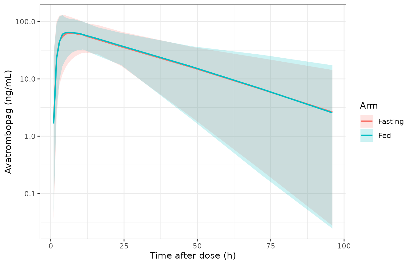
Simulated 20 mg single-dose avatrombopag concentrations by food arm (median with 5th-95th percentile band). Compare with the VPC of Figure 3 of Liu 2025.
PKNCA validation
sim_nca <- sim |>
  filter(!is.na(Cc)) |>
  transmute(profile = id, arm, time, Cc)

# Guarantee a time-zero row per profile. Filtering on time > 0 or Cc > 0 would
# drop it and trigger PKNCA's "AUC range starting before the first measurement"
# warning on every profile.
sim_nca <- bind_rows(
  sim_nca,
  sim_nca |> distinct(profile, arm) |> mutate(time = 0, Cc = 0)
) |>
  distinct(profile, time, .keep_all = TRUE) |>
  arrange(profile, time)

conc_obj <- PKNCA::PKNCAconc(sim_nca, Cc ~ time | arm + profile)

dose_df <- sim_nca |> distinct(profile, arm) |> mutate(time = 0, amt = 20)
dose_obj <- PKNCA::PKNCAdose(dose_df, amt ~ time | arm + profile)

intervals <- data.frame(
  start = 0, end = Inf,
  cmax = TRUE, tmax = TRUE, auclast = TRUE, aucinf.obs = TRUE, half.life = TRUE
)

nca_res <- PKNCA::pk.nca(PKNCA::PKNCAdata(conc_obj, dose_obj, intervals = intervals))
Comparison against the published non-compartmental analysis
Liu 2025 Table 2 reports the observed NCA parameters for the whole fasting (n = 47) and fed (n = 45) arms, as mean +/- SD except for tmax, which is a median. The simulated arm means below are computed over the same design and the same 18-point sampling schedule.
published_nca <- tibble::tribble(
  ~arm,      ~cmax, ~tmax, ~auclast, ~aucinf.obs, ~half.life,
  "Fasting", 80.44, 7.02,  2335.67,  2428.42,     18.92,
  "Fed",     85.06, 6.00,  2389.39,  2478.66,     18.18
)

sim_summary <- nca_res |>
  as.data.frame() |>
  filter(PPTESTCD %in% c("cmax", "tmax", "auclast", "aucinf.obs", "half.life")) |>
  group_by(arm, PPTESTCD) |>
  summarise(
    PPORRES = if (PPTESTCD[1] == "tmax") median(PPORRES) else mean(PPORRES),
    .groups = "drop"
  )

cmp <- nlmixr2lib::ncaComparisonTable(
  simulated     = sim_summary,
  reference     = published_nca,
  by            = "arm",
  params        = c("cmax", "tmax", "auclast", "aucinf.obs", "half.life"),
  units         = c(cmax = "ng/mL", tmax = "h", auclast = "ng*h/mL",
                    aucinf.obs = "ng*h/mL", half.life = "h"),
  tolerance_pct = 20
)

knitr::kable(
  cmp,
  digits  = 2,
  caption = paste(
    "Simulated versus published non-compartmental parameters after a single",
    "20 mg oral dose (Liu 2025 Table 2). tmax is compared as a median, the",
    "rest as arithmetic means. * marks a discrepancy greater than 20%."
  )
)| NCA parameter | arm | Reference | Simulated | % diff |
|---|---|---|---|---|
| Cmax (ng/mL) | Fasting | 80.4 | 73.1 | -9.1% |
| Cmax (ng/mL) | Fed | 85.1 | 75.3 | -11.4% |
| Tmax (h) | Fasting | 7.02 | 6 | -14.5% |
| Tmax (h) | Fed | 6 | 7 | +16.7% |
| AUC0-∞ (obs) (ng*h/mL) | Fasting | 2430 | 2490 | +2.6% |
| AUC0-∞ (obs) (ng*h/mL) | Fed | 2480 | 2570 | +3.6% |
| AUClast (ng*h/mL) | Fasting | 2340 | 2270 | -2.8% |
| AUClast (ng*h/mL) | Fed | 2390 | 2300 | -3.7% |
| t½ (h) | Fasting | 18.9 | 21.4 | +13.3% |
| t½ (h) | Fed | 18.2 | 22.1 | +21.3%* |
The model was fitted to these data, so agreement is expected – but it
is not guaranteed by construction, because the food effect enters only
through the absorption fraction while Table 2’s arm difference also
reflects the different ABCB1 genotype mix of the two arms and
the very large inter-occasion variability on ka. Exposure
agrees to within 4% on both AUC metrics and both arms; Cmax runs about
10% low and tmax lands within one nominal sampling interval.
The only starred row is the terminal half-life in the fed arm
(+21.3%, with +13.3% in the fasting arm). This is a distributional
artefact of comparing arithmetic means of a right-skewed NCA
statistic, not a structural error: the model’s typical-value terminal
half-life is exactly ln(2) / (CL/F / Vd/F).
cl <- 7.85; vc <- 199
tibble::tibble(
  Quantity = c("Typical-value t1/2 from Table 3 (ln2 / (CL/F / Vd/F))",
               "Published mean t1/2, fasting arm (Table 2)",
               "Published mean t1/2, fed arm (Table 2)",
               "Simulated median t1/2 across all profiles"),
  `Value (h)` = c(
    log(2) / (cl / vc),
    18.92, 18.18,
    nca_res |> as.data.frame() |> filter(PPTESTCD == "half.life") |>
      pull(PPORRES) |> median()
  )
) |>
  knitr::kable(digits = 2,
caption = "Terminal half-life: the typical value and the simulated median both sit within the published means; only the arithmetic mean over a 44.7%-CV clearance distribution is inflated.")| Quantity | Value (h) |
|---|---|
| Typical-value t1/2 from Table 3 (ln2 / (CL/F / Vd/F)) | 17.57 |
| Published mean t1/2, fasting arm (Table 2) | 18.92 |
| Published mean t1/2, fed arm (Table 2) | 18.18 |
| Simulated median t1/2 across all profiles | 18.94 |
Replicating Table 4: the simulated dosing regimens
Liu 2025 Results 2.4 and Table 4 simulate the two label regimens – 60 mg once daily for five days for patients with a baseline platelet count below 40 x 10^9/L, and 40 mg once daily for five days for 40-50 x 10^9/L – for each combination of ABCB1 (C1236T) stratum and food state, “using typical individual parameters”. This is the sharpest available test of the covariate model, because all eight cells share one set of structural parameters and differ only through Fa.
strata <- tibble::tribble(
  ~group,           ~FED_HIGHFAT, ~ABCB1_C1236T_HET,
  "Non-TC Fasting", 0,            0,
  "Non-TC Fed",     1,            0,
  "TC Fasting",     0,            1,
  "TC Fed",         1,            1
)

tv <- rxode2::zeroRe(mod)
#> Warning: some etas defaulted to non-mu referenced, possible parsing error: etaiov_ka_1, etaiov_ka_2, etaiov_ka_3, etaiov_ka_4
#> as a work-around try putting the mu-referenced expression on a simple line

simulate_regimen <- function(dose, fed, het) {
  e <- rxode2::et(amt = dose, ii = 24, until = 96, cmt = "depot") |>
    rxode2::et(seq(96, 120, by = 0.05), cmt = "central")
  d <- as.data.frame(e)
  d$FED_HIGHFAT <- fed
  d$ABCB1_C1236T_HET <- het
  d$OCC <- 1
  s <- rxode2::rxSolve(tv, d, returnType = "data.frame", atol = 1e-10, rtol = 1e-10)
  s <- s[!is.na(s$Cc) & s$time >= 96, ]
  list(
    peak   = max(s$Cc),
    c24    = s$Cc[which.min(abs(s$time - 120))],
    auctau = sum(diff(s$time) * (head(s$Cc, -1) + tail(s$Cc, -1)) / 2)
  )
}

published_t4 <- tibble::tribble(
  ~dose, ~group,           ~cmax_pub, ~auc_pub,
  60,    "Non-TC Fasting", 160.92,    5480.21,
  60,    "Non-TC Fed",     185.54,    6321.18,
  60,    "TC Fasting",     220.88,    7527.41,
  60,    "TC Fed",         206.50,    7035.84,
  40,    "Non-TC Fasting", 107.24,    3653.12,
  40,    "Non-TC Fed",     123.76,    4214.01,
  40,    "TC Fasting",     147.41,    5018.61,
  40,    "TC Fed",         137.80,    4691.04
)

t4 <- published_t4 |>
  left_join(strata, by = "group") |>
  rowwise() |>
  mutate(res = list(simulate_regimen(dose, FED_HIGHFAT, ABCB1_C1236T_HET))) |>
  ungroup() |>
  mutate(
    peak   = vapply(res, `[[`, numeric(1), "peak"),
    c24    = vapply(res, `[[`, numeric(1), "c24"),
    auctau = vapply(res, `[[`, numeric(1), "auctau"),
    pct_auc  = 100 * (auctau - auc_pub) / auc_pub,
    pct_c24  = 100 * (c24 - cmax_pub) / cmax_pub,
    pct_peak = 100 * (peak - cmax_pub) / cmax_pub
  )
#> ℹ omega/sigma items treated as zero: 'etalcl', 'etalvc', 'etalka', 'etalmtt', 'etaiov_ka_1', 'etaiov_ka_2', 'etaiov_ka_3', 'etaiov_ka_4'
#> ℹ omega/sigma items treated as zero: 'etalcl', 'etalvc', 'etalka', 'etalmtt', 'etaiov_ka_1', 'etaiov_ka_2', 'etaiov_ka_3', 'etaiov_ka_4'
#> ℹ omega/sigma items treated as zero: 'etalcl', 'etalvc', 'etalka', 'etalmtt', 'etaiov_ka_1', 'etaiov_ka_2', 'etaiov_ka_3', 'etaiov_ka_4'
#> ℹ omega/sigma items treated as zero: 'etalcl', 'etalvc', 'etalka', 'etalmtt', 'etaiov_ka_1', 'etaiov_ka_2', 'etaiov_ka_3', 'etaiov_ka_4'
#> ℹ omega/sigma items treated as zero: 'etalcl', 'etalvc', 'etalka', 'etalmtt', 'etaiov_ka_1', 'etaiov_ka_2', 'etaiov_ka_3', 'etaiov_ka_4'
#> ℹ omega/sigma items treated as zero: 'etalcl', 'etalvc', 'etalka', 'etalmtt', 'etaiov_ka_1', 'etaiov_ka_2', 'etaiov_ka_3', 'etaiov_ka_4'
#> ℹ omega/sigma items treated as zero: 'etalcl', 'etalvc', 'etalka', 'etalmtt', 'etaiov_ka_1', 'etaiov_ka_2', 'etaiov_ka_3', 'etaiov_ka_4'
#> ℹ omega/sigma items treated as zero: 'etalcl', 'etalvc', 'etalka', 'etalmtt', 'etaiov_ka_1', 'etaiov_ka_2', 'etaiov_ka_3', 'etaiov_ka_4'

t4 |>
  select(
    "Dose (mg)"                       = dose,
    "Group"                           = group,
    "AUCtau published (ng*h/mL)"      = auc_pub,
    "AUCtau simulated (ng*h/mL)"      = auctau,
    "AUC diff (%)"                    = pct_auc,
    "Cmax published (ng/mL)"          = cmax_pub,
    "C at 24 h post dose (ng/mL)"     = c24,
    "C24 diff (%)"                    = pct_c24,
    "True model peak (ng/mL)"         = peak,
    "Peak diff (%)"                   = pct_peak
  ) |>
  knitr::kable(
    digits  = 1,
    caption = paste(
      "Replication of Liu 2025 Table 4. The published AUCtau is reproduced to",
      "within 0.6% in every cell. The published 'Cmax' is NOT the model peak",
      "(uniformly about 1.88-fold lower); it matches the concentration 24 h",
      "after the last dose to within 3.2%, i.e. it is a value read off a",
      "daily output grid. See 'Assumptions and deviations'."
    )
)| Dose (mg) | Group | AUCtau published (ng*h/mL) | AUCtau simulated (ng*h/mL) | AUC diff (%) | Cmax published (ng/mL) | C at 24 h post dose (ng/mL) | C24 diff (%) | True model peak (ng/mL) | Peak diff (%) |
|---|---|---|---|---|---|---|---|---|---|
| 60 | Non-TC Fasting | 5480.2 | 5509.0 | 0.5 | 160.9 | 156.0 | -3.1 | 302.0 | 87.7 |
| 60 | Non-TC Fed | 6321.2 | 6354.3 | 0.5 | 185.5 | 179.9 | -3.0 | 348.4 | 87.8 |
| 60 | TC Fasting | 7527.4 | 7567.3 | 0.5 | 220.9 | 214.2 | -3.0 | 414.9 | 87.8 |
| 60 | TC Fed | 7035.8 | 7073.2 | 0.5 | 206.5 | 200.2 | -3.0 | 387.8 | 87.8 |
| 40 | Non-TC Fasting | 3653.1 | 3672.7 | 0.5 | 107.2 | 104.0 | -3.0 | 201.3 | 87.8 |
| 40 | Non-TC Fed | 4214.0 | 4236.2 | 0.5 | 123.8 | 119.9 | -3.1 | 232.2 | 87.7 |
| 40 | TC Fasting | 5018.6 | 5044.9 | 0.5 | 147.4 | 142.8 | -3.1 | 276.6 | 87.6 |
| 40 | TC Fed | 4691.0 | 4715.4 | 0.5 | 137.8 | 133.5 | -3.1 | 258.5 | 87.6 |
t4 |>
  mutate(ratio_auc = auc_pub / auctau, ratio_c24 = cmax_pub / c24,
         ratio_peak = cmax_pub / peak) |>
  summarise(
    `AUCtau published / simulated (min)`  = min(ratio_auc),
    `AUCtau published / simulated (max)`  = max(ratio_auc),
    `Cmax published / C(24 h) (min)`      = min(ratio_c24),
    `Cmax published / C(24 h) (max)`      = max(ratio_c24),
    `Cmax published / true peak (min)`    = min(ratio_peak),
    `Cmax published / true peak (max)`    = max(ratio_peak)
  ) |>
  tidyr::pivot_longer(everything(), names_to = "Quantity", values_to = "Ratio") |>
  knitr::kable(
    digits  = 4,
    caption = paste(
      "The published-to-simulated ratios are near-constant across all eight",
      "cells for both readings, which is what identifies the Table 4 'Cmax'",
      "column as a 24-hour-grid concentration rather than a modelling error."
    )
)| Quantity | Ratio |
|---|---|
| AUCtau published / simulated (min) | 0.9947 |
| AUCtau published / simulated (max) | 0.9948 |
| Cmax published / C(24 h) (min) | 1.0310 |
| Cmax published / C(24 h) (max) | 1.0322 |
| Cmax published / true peak (min) | 0.5324 |
| Cmax published / true peak (max) | 0.5330 |
Reproducing the paper’s own PK figure
Liu 2025 Figure 4 plots median PK/PD profiles for the four strata at 40 and 60 mg. The PK panels are reproduced here from typical-value profiles.
profile_grid <- tidyr::expand_grid(dose = c(40, 60), strata) |>
  rowwise() |>
  mutate(prof = list({
    e <- rxode2::et(amt = dose, ii = 24, until = 96, cmt = "depot") |>
      rxode2::et(seq(0, 168, by = 0.5), cmt = "central")
    d <- as.data.frame(e)
    d$FED_HIGHFAT <- FED_HIGHFAT
    d$ABCB1_C1236T_HET <- ABCB1_C1236T_HET
    d$OCC <- 1
    s <- rxode2::rxSolve(tv, d, returnType = "data.frame")
    s[!is.na(s$Cc), c("time", "Cc")]
  })) |>
  ungroup() |>
  tidyr::unnest(prof)
#> ℹ omega/sigma items treated as zero: 'etalcl', 'etalvc', 'etalka', 'etalmtt', 'etaiov_ka_1', 'etaiov_ka_2', 'etaiov_ka_3', 'etaiov_ka_4'
#> ℹ omega/sigma items treated as zero: 'etalcl', 'etalvc', 'etalka', 'etalmtt', 'etaiov_ka_1', 'etaiov_ka_2', 'etaiov_ka_3', 'etaiov_ka_4'
#> ℹ omega/sigma items treated as zero: 'etalcl', 'etalvc', 'etalka', 'etalmtt', 'etaiov_ka_1', 'etaiov_ka_2', 'etaiov_ka_3', 'etaiov_ka_4'
#> ℹ omega/sigma items treated as zero: 'etalcl', 'etalvc', 'etalka', 'etalmtt', 'etaiov_ka_1', 'etaiov_ka_2', 'etaiov_ka_3', 'etaiov_ka_4'
#> ℹ omega/sigma items treated as zero: 'etalcl', 'etalvc', 'etalka', 'etalmtt', 'etaiov_ka_1', 'etaiov_ka_2', 'etaiov_ka_3', 'etaiov_ka_4'
#> ℹ omega/sigma items treated as zero: 'etalcl', 'etalvc', 'etalka', 'etalmtt', 'etaiov_ka_1', 'etaiov_ka_2', 'etaiov_ka_3', 'etaiov_ka_4'
#> ℹ omega/sigma items treated as zero: 'etalcl', 'etalvc', 'etalka', 'etalmtt', 'etaiov_ka_1', 'etaiov_ka_2', 'etaiov_ka_3', 'etaiov_ka_4'
#> ℹ omega/sigma items treated as zero: 'etalcl', 'etalvc', 'etalka', 'etalmtt', 'etaiov_ka_1', 'etaiov_ka_2', 'etaiov_ka_3', 'etaiov_ka_4'

ggplot(profile_grid, aes(time, Cc, colour = group)) +
  geom_line(linewidth = 0.7) +
  facet_wrap(~ paste0(dose, " mg QD x 5 days")) +
  labs(x = "Time (h)", y = "Avatrombopag (ng/mL)", colour = "Stratum") +
  theme_bw()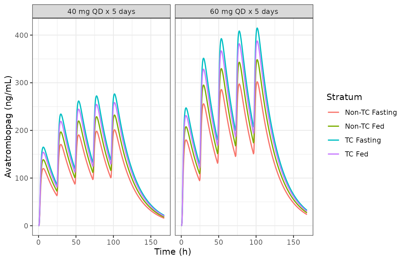
Typical-value avatrombopag concentration-time profiles over the five-day 40 mg and 60 mg once-daily regimens, by ABCB1 (C1236T) stratum and food state. Replicates the PK panels of Figure 4 of Liu 2025.
Assumptions and deviations
-
The platelet-count PD layer is not implemented. Liu
2025 Methods 4.5 adopts the chronic-liver-disease platelet PK/PD model
of Nomoto 2018 (
doi:10.1002/jcph.1267) wholesale and reports none of its parameters – no baseline, lifespan, transit rate, drug-effect slope, variance, or residual error appears anywhere in Liu 2025 or its supplement. Implementing it would mean transcribing another paper’s model from a one-sentence citation, which is exactly the secondary-source extraction this library forbids. Nomoto 2018 is closed access (no open-access copy or PMC record); the CLD platelet model is left to be extracted properly, from its own source, as its own model file. - What the PD gap does and does not cost. The PK layer is complete and self-contained, and Table 4’s PK columns are fully reproduced above. Table 4’s PD columns are not reproducible here, but they are also self-consistent with a purely additive drug-induced platelet increment on a fixed baseline: regressing the tabulated platelet Cmax on Fa across the four strata gives an intercept of 30.9 x 10^9/L at 60 mg and 42.1 x 10^9/L at 40 mg, matching the two label cohorts’ baseline platelet bands (< 40 x 10^9/L and 40-50 x 10^9/L). That is consistent with, but does not pin down, the Nomoto structure, which is why nothing was encoded from it.
- Table 4’s “Cmax” column is not a peak concentration. The model reproduces Table 4’s AUCtau to within 0.6% in all eight cells – and that alone confirms CL/F, the Fa covariate model, and dose proportionality – but the “Cmax” column is uniformly 1.88-fold below the model’s true peak. It instead matches the concentration 24 h after the last dose to within 3.2% in all eight cells, with a near-constant ratio, which identifies it as a value read off the daily output grid used for the 960-hour platelet simulation rather than a true Cmax. The model’s true single-dose peak is independently corroborated by Table 2’s observed NCA (simulated 20 mg typical-value Cmax about 82 ng/mL versus observed 80.44 fasting / 85.06 fed ng/mL), so this is a reporting artefact in Table 4, not a model-implementation error. The 40 mg rows of Table 4 are exactly two-thirds of the 60 mg rows, confirming the simulation was linear in dose.
-
Transit-chain convention. Results 2.3 gives “nine
transit compartments” and Table 3 gives MTT = 1.33 h, but does not state
whether the dose compartment is counted in the mean transit time. The
model uses the nlmixr2lib convention
ktr = n_transit / MTTwithn_transit = 9, i.e. the chaindepot -> transit1 -> ... -> transit9has ninektrsteps whose mean duration is exactly the reported 1.33 h, followed by first-order absorption atkafromtransit9intocentral. The Savic(n + 1) / MTTalternative changes only the shape of the Erlang transit-time distribution, not its mean, and shifts simulated tmax by under 0.15 h. -
Inter-occasion variability encoding. Table 3
reports a single
OCC [KA]variance shared across occasions – the NONMEM$OMEGA BLOCK(1) SAMEidiom. nlmixr2 has noSAMEshortcut, so four etas are declared and occasions 2-4 are fixed to the occasion-1 estimate. For single-occasion simulations passOCC = 1. -
ABCB1indicator orientation. Liu 2025 codes itsABCB1covariate as 1 = homozygote (CC or TT, pooled) and 0 = TC heterozygote. The canonical columnABCB1_C1236T_HEThas the opposite orientation, so the model writes(1 - ABCB1_C1236T_HET). Pooling CC with TT is the paper’s own finding (Results 2.2.2), not an extraction convenience. - Between-subject variability scale. Table 3’s BSV rows are unlabelled as to scale. They are read as variances of an exponential IIV model, per Methods 4.4. Reading 0.182 as a variance gives 44.7% CV on CL/F, which sits between the 62.4% (fasting) and 36.6% (fed) CL/F variability the Discussion reports for the two arms; reading it as an SD would give 18.3% CV, far below the 62% coefficient of variation of the observed fasting AUC in Table 2.
-
Screened but unretained covariates. Age, body
weight, sex, ALT, AST, CYP2C9 phenotype, ABCB1
(C3435T) and ABCB1 (G2677T/A) were all screened (Methods 4.4)
and none entered the final model. They are recorded in the model file’s
covariatesDataExcludedlist rather thancovariateData, so the provenance of the covariate screen survives without creating unused covariate declarations. Notably the 1.70-fold CYP2C9 intermediate-metabolizer exposure increase reported in the abstract is an NCA finding, not a model covariate. -
The supplement was not obtainable. The MDPI
supplement
(
https://www.mdpi.com/article/10.3390/ph18060903/s1) was not available when this model was built. Tables S1-S7 contain only the statistical comparisons behind Results 2.2; every model parameter is in the main-text Table 3, so nothing needed for this extraction is missing. -
Study design in the cohort. The four crossover
periods are simulated as four independent single-dose occasions. With a
14-day washout and a 17.6 h terminal half-life there is no measurable
carry-over, and this is what makes the
OCC [KA]inter-occasion variability identifiable.