Model and source
- Citation: Jang Y, Ahn SJ, Lee S, Kim Y, Lee HS, Lee YK, Shin YW, Lee ST, Jung KH, Park KI, Jung KY, Cho JY, Lee S, Yu KS, Chu K, Jang IJ, Lee SK. Saliva-based lacosamide monitoring paves the way toward personalized epilepsy pharmacotherapy. Sci Rep. 2025;15:19181. doi:10.1038/s41598-025-04044-x. PMCID: PMC12126552.
- Description: One-compartment population PK model with first-order absorption for oral lacosamide in Korean adults with epilepsy, fit jointly to plasma/serum and saliva concentrations: saliva is the plasma concentration times an estimated saliva:plasma scale factor of 1.44; CYP2C19 poor-metabolizer phenotype, concomitant carbamazepine and phenobarbital, and creatinine clearance on apparent clearance; body surface area on apparent volume
- Article: https://doi.org/10.1038/s41598-025-04044-x (open access; the model parameters are in Supplementary Table 2 of the Supplementary Information)
Jang et al. measured lacosamide in paired plasma/serum and unstimulated saliva from adults with epilepsy and fit a one-compartment population PK model to both matrices together. Saliva is not a separate kinetic compartment: the saliva concentration is the plasma concentration times an estimated scale factor of 1.44 (Figure 2A). The model was then used to estimate each patient’s steady-state saliva peak and trough and to derive saliva cutoffs for seizure control (15.94 mg/L for the peak, 9.056 mg/L for the trough; Figure 3).
Population
The analysis included 123 Korean outpatients with epilepsy treated at Seoul National University Hospital between August 2021 and November 2022 (Table 1): mean age 41.3 +/- 14.2 years, 54.5% male, body weight 67.2 +/- 14.3 kg, body surface area 1.8 +/- 0.2 m^2. Seizures were focal in 91.9% of patients. All patients took lacosamide twice daily on a regimen unchanged for at least one month (median total daily dose 300 mg, IQR 200-400), and 63.1% took other antiseizure medications. Renal function was normal (serum creatinine 0.8 +/- 0.1 mg/dL, GFR 101 +/- 19 mL/min/1.73 m^2). CYP2C19 was genotyped in 37 patients: 13 normal, 18 intermediate and 6 poor metabolizers.
The PK dataset held 109 spot saliva samples, 59 saliva samples the patients collected themselves at home, and 102 blood samples from 86 patients, drawn a median of 4.25 h (saliva) and 4.67 h (blood) after the last dose. Because the sampling was sparse, the absorption rate constant, the apparent volume and the body-surface-area exponent on the volume were fixed to the healthy Korean volunteer model of Kim et al. (Pharmacology 2012;89:172).
The same information is available programmatically via
readModelDb("Jang_2025_lacosamide")()$population.
Source trace
| Equation / parameter | Value | Source location |
|---|---|---|
lcl (CL/F, CYP2C19 normal + intermediate) |
log(1.78) L/h | Supplementary Table 2, theta1 (RSE 3.0%); Results |
e_cyp2c19_pm_cl |
1.43 / 1.78 | Supplementary Table 2, theta2 = 1.43 L/h (RSE 7.4%) over theta1 |
e_conmed_cbz_cl |
0.771 | Supplementary Table 2, theta3 (RSE 35.4%); Results |
e_conmed_pb_cl |
0.467 | Supplementary Table 2, theta4 (RSE 45.6%); Results |
e_crcl_cl |
0.579 | Supplementary Table 2, theta5 (RSE 13.7%); Results |
lvc (V/F) |
fixed(log(41.6)) L | Supplementary Table 2, theta6 (fixed; Methods) |
e_bsa_vc |
fixed(1.37) | Supplementary Table 2, theta7 (fixed; Methods) |
lka |
fixed(log(6.47)) 1/h | Supplementary Table 2, theta8 (fixed; Methods) |
lfsaliva |
log(1.44) | Supplementary Table 2, theta9 (RSE 4.0%); Results; Discussion |
etalcl |
0.05510 = log(1 + 0.238^2) | Supplementary Table 2, omega CL/F = 23.8 %CV |
propSd (blood) |
0.270 | Supplementary Table 2, sigma blood,prop |
propSd_Csaliva |
0.407 | Supplementary Table 2, sigma saliva,prop |
| CL/F equation | (theta1 or theta2) * (1 + theta3*CBZ + theta4*PB) * (CLcr/107)^theta5 |
Supplementary Table 2 structure row; Results |
| V/F equation | theta6 * (BSA/1.856)^theta7 |
Supplementary Table 2 structure row |
| One compartment, first-order absorption |
d/dt(depot), d/dt(central)
|
Figure 2A; Results |
| Saliva concentration | Csaliva = fsaliva * Cc |
Figure 2A; Results |
Typical-value check against the closed form
For a one-compartment model with first-order absorption at steady
state, the concentration at time t after a dose
D given every tau hours is
D*ka/(V*(ka-k)) * (exp(-k t)/(1-exp(-k tau)) - exp(-ka t)/(1-exp(-ka tau))).
The packaged model is solved numerically; the comparison below confirms
the ODEs, the covariate reference values and the saliva scale
factor.
mod <- readModelDb("Jang_2025_lacosamide")
mod_typ <- rxode2::zeroRe(mod)
#> ℹ parameter labels from comments will be replaced by 'label()'

# Reference patient: CYP2C19 normal/intermediate metabolizer, no inducer,
# CRCL 107 mL/min and BSA 1.856 m^2, i.e. every covariate term equal to 1.
tau <- 12
dose <- 150
ss_start <- 27 * tau
typ_events <- data.frame(
  id = 1L,
  time = c(seq(0, ss_start, by = tau), ss_start + seq(0.25, tau, by = 0.25)),
  evid = c(rep(1L, 28), rep(0L, 48)),
  amt = c(rep(dose, 28), rep(0, 48)),
  cmt = c(rep("depot", 28), rep("central", 48)),
  # dvid 1 = the plasma endpoint Cc; Csaliva is returned on the same rows.
  dvid = c(rep(NA_integer_, 28), rep(1L, 48)),
  BSA = 1.856, CRCL = 107, CYP2C19_PM = 0L, CONMED_CBZ = 0L, CONMED_PB = 0L
)
typ <- as.data.frame(rxode2::rxSolve(mod_typ, events = typ_events,
                                     atol = 1e-10, rtol = 1e-10))
#> ℹ omega/sigma items treated as zero: 'etalcl'

ka <- 6.47; vc <- 41.6; k <- 1.78 / vc
tad <- typ$time - ss_start
closed <- dose * ka / (vc * (ka - k)) *
  (exp(-k * tad) / (1 - exp(-k * tau)) - exp(-ka * tad) / (1 - exp(-ka * tau)))
rel_err <- max(abs(typ$Cc - closed) / closed)
rel_err
#> [1] 6.203399e-07
stopifnot(rel_err < 1e-5)
# Saliva is an exact algebraic rescaling of the plasma concentration.
stopifnot(max(abs(typ$Csaliva / typ$Cc - 1.44)) < 1e-8)
# AUC over a dosing interval at steady state equals dose / CL.
dose / 1.78
#> [1] 84.26966
At 150 mg twice daily the reference patient’s steady-state AUC over a dosing interval is 84.3 mg h/L in blood and 121.3 mg h/L in saliva. Table 1 reports cohort means of 83.7 and 120 mg h/L for the model-estimated individual AUCs, at a median dose of 300 mg/day.
Virtual cohort
Observed data are not public. The virtual cohort below reproduces the Table 1 demographics where the paper reports them and uses stated assumptions where it does not (see Assumptions and deviations).
rxode2::rxSetSeed(20250531)
set.seed(20250531)

# Steady-state dosing train: 28 twice-daily doses, then one dosing interval
# observed every 15 min. The half-life of the reference patient is about 16 h,
# so 13.5 days of dosing is past steady state.
make_cohort <- function(n, daily_dose, id_offset = 0L, cohort = "Table 1") {
  subj <- tibble(
    id = id_offset + seq_len(n),
    cohort = cohort,
    daily_dose = daily_dose,
    BSA = pmin(pmax(rnorm(n, 1.8, 0.2), 1.3), 2.4),
    # Raw creatinine clearance in mL/min centred on the 107 mL/min reference.
    CRCL = 107 * exp(rnorm(n, 0, 0.2)),
    CYP2C19_PM = rbinom(n, 1, 6 / 37),
    CONMED_CBZ = rbinom(n, 1, 0.10),
    CONMED_PB = rbinom(n, 1, 0.05)
  )
  doses <- subj |>
    tidyr::expand_grid(time = seq(0, ss_start, by = tau)) |>
    mutate(evid = 1L, amt = daily_dose / 2, cmt = "depot", dvid = NA_integer_)
  obs <- subj |>
    tidyr::expand_grid(time = ss_start + seq(0, tau, by = 0.25)) |>
    mutate(evid = 0L, amt = 0, cmt = "central", dvid = 1L)
  bind_rows(doses, obs) |> arrange(id, time, desc(evid))
}

# Table 1 cohort: total daily dose drawn to give the reported median 300 mg
# and IQR 200-400 mg.
n_tab <- 200
dose_tab <- sample(c(100, 200, 300, 400, 500, 600), n_tab, replace = TRUE,
                   prob = c(0.05, 0.30, 0.25, 0.30, 0.05, 0.05))
events_tab <- make_cohort(n_tab, dose_tab)

# Fixed-dose arms for the saliva cutoff comparison (Figure 3).
arm_doses <- c(200, 300, 400, 500, 600)
events_arms <- bind_rows(lapply(seq_along(arm_doses), function(i) {
  make_cohort(200, arm_doses[i], id_offset = n_tab + (i - 1L) * 200L,
              cohort = paste(arm_doses[i], "mg/day"))
}))
events <- bind_rows(events_tab, events_arms)
stopifnot(!anyDuplicated(unique(events[, c("id", "time", "evid")])))
summary(dose_tab)
#>    Min. 1st Qu.  Median    Mean 3rd Qu.    Max.
#>   100.0   200.0   300.0   306.5   400.0   600.0
Simulation
sim <- rxode2::rxSolve(mod, events = events,
                       keep = c("cohort", "daily_dose")) |>
  as.data.frame()
#> ℹ parameter labels from comments will be replaced by 'label()'
sim_tab <- filter(sim, cohort == "Table 1")
PKNCA validation against Table 1
Table 1 (and the text under Figure 2) reports the mean +/- SD of each patient’s model-estimated steady-state peak, trough and AUC in blood and saliva. The same quantities are computed with PKNCA over the last simulated dosing interval, once per matrix.
nca_one <- function(sim, conc_col, matrix_label) {
  conc <- sim |>
    filter(!is.na(.data[[conc_col]])) |>
    transmute(id, time, conc = .data[[conc_col]], matrix = matrix_label)
  dose_df <- events_tab |>
    filter(evid == 1, time == ss_start) |>
    transmute(id, time, amt, matrix = matrix_label)
  conc_obj <- PKNCA::PKNCAconc(conc, conc ~ time | matrix + id)
  dose_obj <- PKNCA::PKNCAdose(dose_df, amt ~ time | matrix + id)
  intervals <- data.frame(start = ss_start, end = ss_start + tau,
                          cmax = TRUE, cmin = TRUE, auclast = TRUE)
  PKNCA::pk.nca(PKNCA::PKNCAdata(conc_obj, dose_obj, intervals = intervals))
}
nca_blood <- nca_one(sim_tab, "Cc", "blood")
nca_saliva <- nca_one(sim_tab, "Csaliva", "saliva")

nca_ind <- bind_rows(as.data.frame(nca_blood), as.data.frame(nca_saliva))

# Table 1 reports MEANS of the individual estimates, so the simulated values
# are summarised by the mean as well (ncaComparisonTable() would otherwise
# take the median).
sim_means <- nca_ind |>
  group_by(matrix, PPTESTCD) |>
  summarise(PPORRES = mean(PPORRES), .groups = "drop")

published <- tibble::tribble(
  ~matrix,  ~cmax, ~cmin, ~auclast,
  "blood",   8.89,  5.25,     83.7,
  "saliva",  12.8,  7.56,      120
)

cmp <- nlmixr2lib::ncaComparisonTable(
  simulated = sim_means,
  reference = published,
  by = "matrix",
  units = c(cmax = "mg/L", cmin = "mg/L", auclast = "mg*h/L"),
  tolerance_pct = 20
)
knitr::kable(cmp, caption = paste(
  "Simulated vs. published (Table 1) steady-state exposure, mean over the",
  "cohort. Trough = Cmin over the dosing interval. * differs from the",
  "reference by more than 20%."
))| NCA parameter | matrix | Reference | Simulated | % diff |
|---|---|---|---|---|
| Cmax (mg/L) | blood | 8.89 | 9.32 | +4.9% |
| Cmax (mg/L) | saliva | 12.8 | 13.4 | +4.9% |
| Cmin (mg/L) | blood | 5.25 | 5.71 | +8.7% |
| Cmin (mg/L) | saliva | 7.56 | 8.22 | +8.7% |
| AUClast (mg*h/L) | blood | 83.7 | 89.2 | +6.6% |
| AUClast (mg*h/L) | saliva | 120 | 128 | +7.0% |
pct <- function(code, m) {
  s <- sim_means$PPORRES[sim_means$PPTESTCD == code & sim_means$matrix == m]
  r <- published[[code]][published$matrix == m]
  stopifnot(length(s) == 1L, length(r) == 1L)
  100 * (s - r) / r
}
pct_all <- c(
  sapply(c("cmax", "cmin", "auclast"), pct, m = "blood"),
  sapply(c("cmax", "cmin", "auclast"), pct, m = "saliva")
)
round(pct_all, 1)
#>    cmax    cmin auclast    cmax    cmin auclast
#>     4.9     8.7     6.6     4.9     8.7     7.0
# Cohort means of 200 subjects: the AUC SD in Table 1 (37%) gives a standard
# error near 3%, so 20% leaves room for the assumed dose and inducer mix and
# still fails on a misread clearance, volume or scale factor.
stopifnot(all(abs(pct_all) < 20))
Replicate published figures
Figure 1C: saliva versus blood concentration
Figure 1C regresses 74 paired saliva and blood concentrations,
sampled a median of about 4.5 h after the dose, and reports
Csaliva = 4.932 + 0.652 * Cblood (adjusted R^2 0.38). The
model instead predicts a ratio of 1.44 through the origin. Adding each
matrix’s proportional residual error to simulated paired samples shows
how much of the flatter published slope is regression dilution from
measurement noise in the blood concentration.
# One paired sample per patient at a time after dose drawn around the
# Table 1 medians (4.25 h saliva, 4.67 h blood), on the 15-min grid.
samp <- tibble(
  id = unique(sim_tab$id),
  tad = round(4 * pmin(pmax(rlnorm(n_tab, log(4.5), 0.5), 0.25), 12)) / 4
)
pairs <- sim_tab |>
  mutate(tad = time - ss_start) |>
  inner_join(samp, by = c("id", "tad")) |>
  mutate(
    blood_obs = Cc * (1 + 0.270 * rnorm(n())),
    saliva_obs = Csaliva * (1 + 0.407 * rnorm(n()))
  )
stopifnot(nrow(pairs) == n_tab)
fit <- lm(saliva_obs ~ blood_obs, data = pairs)
coef(fit)
#> (Intercept)   blood_obs
#>    1.817941    1.184081

ggplot(pairs, aes(blood_obs, saliva_obs)) +
  geom_point(alpha = 0.5) +
  geom_abline(intercept = 4.932, slope = 0.652, colour = "firebrick") +
  geom_abline(intercept = 0, slope = 1.44, linetype = "dashed") +
  geom_smooth(method = "lm", formula = y ~ x, se = FALSE, colour = "steelblue") +
  labs(x = "Blood lacosamide (mg/L)", y = "Saliva lacosamide (mg/L)",
       title = "Simulated paired samples with residual error",
       caption = paste(
         "Replicates Figure 1C of Jang 2025. Red: published regression;",
         "dashed: model ratio 1.44; blue: regression on the simulated pairs."
       ))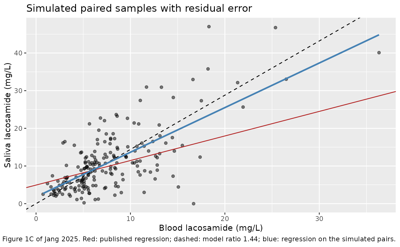
Regressing the simulated pairs gives an intercept of 1.82 mg/L and a slope of 1.18. Measurement noise therefore flattens the slope below 1.44 but does not account for all of the published 0.652. The rest is not reproduced by the model. The paper’s pairs differ from the simulation in ways the model does not represent: blood and saliva were collected up to 30 minutes apart, blood came from plasma and serum tubes analysed together, and the regression used only the 74 patients who gave both samples. The model’s ratio of 1.44 is the paper’s own estimate (Supplementary Table 2) and is the value used for the saliva cutoffs.
Figure 1D: CYP2C19 phenotype
Figure 1D shows dose-normalised blood concentrations rising from normal to intermediate to poor metabolizers. The final model pools normal and intermediate metabolizers, so poor metabolizers are predicted to have 1.78 / 1.43 = 1.245 times the exposure of everyone else.
sim_tab |>
  mutate(tad = time - ss_start,
         Cc_dn = Cc * 300 / daily_dose,
         phenotype = ifelse(CYP2C19_PM == 1, "Poor", "Normal or intermediate")) |>
  filter(abs(tad - 4.5) < 0.01) |>
  ggplot(aes(phenotype, Cc_dn)) +
  geom_boxplot() +
  labs(x = "CYP2C19 phenotype",
       y = "Dose-normalised blood lacosamide at 4.5 h (mg/L per 300 mg/day)",
       caption = "Replicates the structure of Figure 1D of Jang 2025.")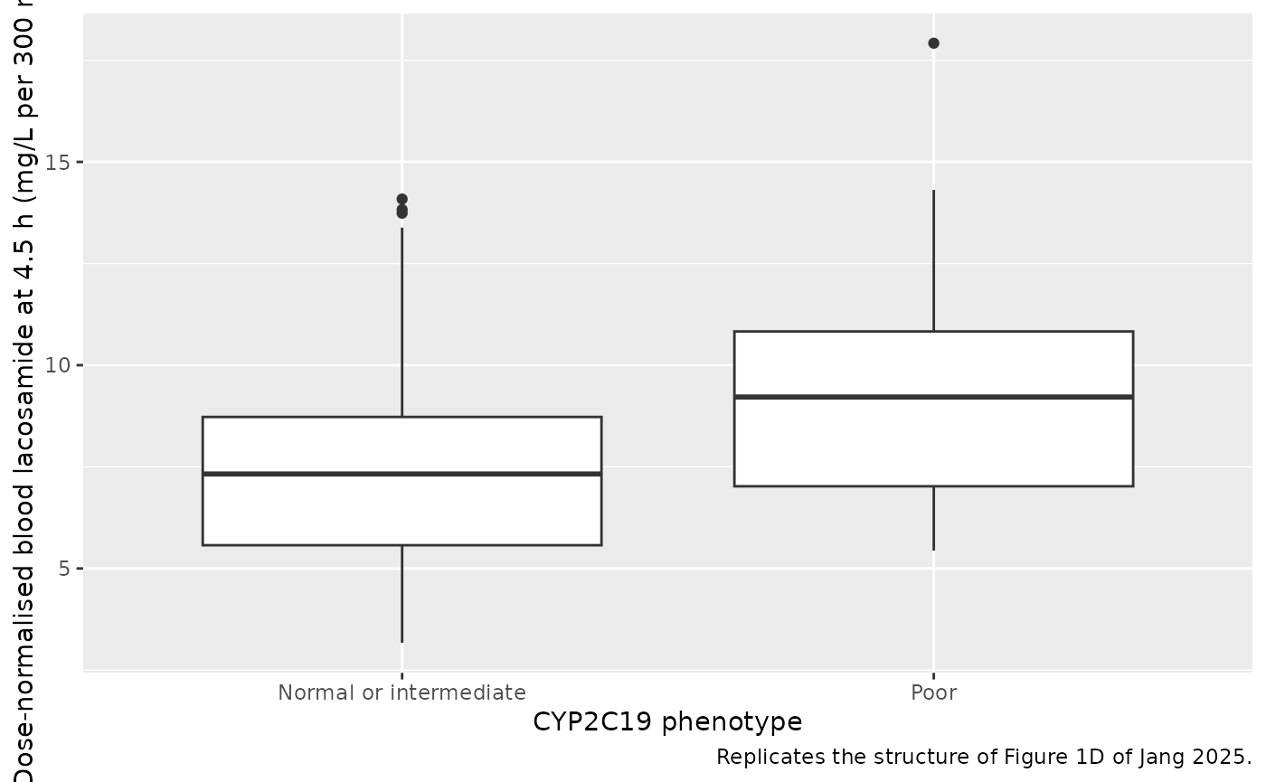
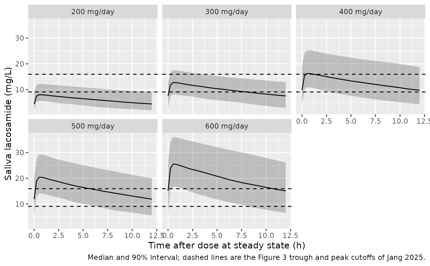
Figure 3: saliva cutoffs by daily dose
Figure 3 identifies a steady-state saliva peak of 15.94 mg/L and trough of 9.056 mg/L as the best cutoffs for well-controlled seizures in the high seizure burden group, and Supplementary Table 5 reports estimated saliva peaks of 16.51 +/- 4.24 mg/L and troughs of 10.32 +/- 3.18 mg/L at a median daily dose of 400 mg once control was achieved. The fixed-dose arms show how often each daily dose reaches the cutoffs.
arm_summary <- sim |>
  filter(cohort != "Table 1") |>
  group_by(cohort, daily_dose, id) |>
  summarise(peak = max(Csaliva), trough = Csaliva[time == ss_start + tau],
            .groups = "drop") |>
  group_by(daily_dose) |>
  summarise(
    peak_mean = mean(peak), peak_sd = sd(peak),
    trough_mean = mean(trough), trough_sd = sd(trough),
    pct_peak_over = 100 * mean(peak > 15.94),
    pct_trough_over = 100 * mean(trough > 9.056),
    .groups = "drop"
  )
arm_summary |>
  dplyr::rename(
    "Daily dose (mg)" = daily_dose,
    "Saliva peak mean (mg/L)" = peak_mean,
    "Saliva peak SD" = peak_sd,
    "Saliva trough mean (mg/L)" = trough_mean,
    "Saliva trough SD" = trough_sd,
    "% peak > 15.94" = pct_peak_over,
    "% trough > 9.056" = pct_trough_over
  ) |>
  knitr::kable(digits = 1, caption = paste(
    "Simulated steady-state saliva exposure by daily dose (200 virtual",
    "patients per arm)."
))| Daily dose (mg) | Saliva peak mean (mg/L) | Saliva peak SD | Saliva trough mean (mg/L) | Saliva trough SD | % peak > 15.94 | % trough > 9.056 |
|---|---|---|---|---|---|---|
| 200 | 8.3 | 2.1 | 4.9 | 2.1 | 1.0 | 3.5 |
| 300 | 12.9 | 3.0 | 7.8 | 3.1 | 15.5 | 31.5 |
| 400 | 17.2 | 4.3 | 10.4 | 4.3 | 55.5 | 56.5 |
| 500 | 20.9 | 4.7 | 12.3 | 4.6 | 86.5 | 79.0 |
| 600 | 25.9 | 6.2 | 15.7 | 6.2 | 97.0 | 87.0 |
at400 <- arm_summary[arm_summary$daily_dose == 400, ]
stopifnot(nrow(at400) == 1L)
# Supplementary Table 5: 16.51 mg/L peak and 10.32 mg/L trough at a median of
# 400 mg/day. The structural check is on the cohort mean.
stopifnot(abs(at400$peak_mean / 16.51 - 1) < 0.2,
          abs(at400$trough_mean / 10.32 - 1) < 0.2)

sim |>
  filter(cohort != "Table 1") |>
  mutate(tad = time - ss_start) |>
  group_by(cohort, daily_dose, tad) |>
  summarise(Q05 = quantile(Csaliva, 0.05), Q50 = median(Csaliva),
            Q95 = quantile(Csaliva, 0.95), .groups = "drop") |>
  ggplot(aes(tad, Q50)) +
  geom_ribbon(aes(ymin = Q05, ymax = Q95), alpha = 0.25) +
  geom_line() +
  geom_hline(yintercept = c(9.056, 15.94), linetype = "dashed") +
  facet_wrap(~ reorder(cohort, daily_dose)) +
  labs(x = "Time after dose at steady state (h)",
       y = "Saliva lacosamide (mg/L)",
       caption = paste(
         "Median and 90% interval; dashed lines are the Figure 3 trough and",
         "peak cutoffs of Jang 2025."
       ))
Assumptions and deviations
- CYP2C19 poor-metabolizer clearance. The paper estimates a separate typical CL/F for poor metabolizers (1.43 L/h). The model carries it as the factor 1.43/1.78 on the pooled normal-plus-intermediate clearance, which gives the same typical values. Only 37 of the 123 patients were genotyped and the paper does not say how the others were handled; the virtual cohort draws the poor-metabolizer phenotype at the genotyped frequency (6/37).
- Creatinine clearance. The paper does not state how CLcr was calculated. It is supplied in mL/min (not BSA-normalised) because the covariate equation is normalised by 107 mL/min. The virtual cohort draws CRCL log-normally around 107 mL/min with a 20% spread, consistent with the Table 1 GFR of 101 +/- 19 mL/min/1.73 m^2 and BSA of 1.8 m^2.
- Concomitant carbamazepine and phenobarbital. The paper reports that 63.1% of patients took other antiseizure medications but not how many took carbamazepine or phenobarbital. The virtual cohort assumes 10% and 5%.
- Dose distribution. Table 1 gives only the median (300 mg/day) and IQR (200-400 mg/day); the virtual Table 1 cohort draws doses of 100-600 mg/day to match these.
- Residual error scale. Supplementary Table 2 prints the residual errors as 0.270 (blood) and 0.407 (saliva) without stating the scale. They are treated as standard deviations: the bootstrap 95% intervals have relative widths of 0.28 and 0.22, matching the width expected for a standard deviation estimated from 102 and 168 samples (0.27 and 0.21) and half the width expected for a variance, and the RSEs (7.3% and 6.5%) agree.
- Inter-individual variability. The 23.8% CV on CL/F is converted to a log-normal variance as log(1 + 0.238^2) = 0.0551.
-
Blood matrix. Blood concentrations came from plasma
and serum tubes analysed together;
Ccrepresents both. - No correction notice for this article was found on Europe PMC as of 2026-11-04.