Piperacillin (Tseng 2026)
Source:vignettes/articles/Tseng_2026_piperacillin.Rmd
Tseng_2026_piperacillin.RmdModel and source
ui <- rxode2::rxode(readModelDb("Tseng_2026_piperacillin"))
#> ℹ parameter labels from comments will be replaced by 'label()'- Citation: Tseng YJ, Juan L, Tai CH, Wu CC. Optimal piperacillin/tazobactam dosing in adults with low body weight: a population pharmacokinetic and simulation-based study. Drug Des Devel Ther. 2026;20:1-12. doi:10.2147/DDDT.S602835. PMCID: PMC13157127.
- Description: One-compartment population PK model for piperacillin in adults with low body weight (BMI <= 18.5 kg/m^2) receiving piperacillin-tazobactam (Tseng 2026). Clearance is scaled by a power function of the 2021 CKD-EPI creatinine-cystatin C estimated glomerular filtration rate; body weight was screened and not retained. Interindividual variability is carried on clearance only, the volume random effect having been removed for 83.2% shrinkage. A fixed unbound fraction of 0.7 converts the modelled total plasma concentration to the free concentration that drives the paper’s 100% fT > MIC target-attainment simulations.
- Article: https://doi.org/10.2147/DDDT.S602835
Tseng and colleagues developed a one-compartment population PK model for piperacillin in hospitalised adults with low body weight (LBW, body mass index at or below 18.5 kg/m^2), then used it to compare intermittent against prolonged infusion across renal-function strata. The paper’s headline negative finding is that body weight did not improve the fit once renal function was accounted for; its headline positive finding is that renal function, best described by the 2021 CKD-EPI combined creatinine-cystatin C equation, is the dominant determinant of piperacillin clearance in this population.
Population
The analysis dataset comprises 55 plasma samples from 29 adults enrolled prospectively at National Taiwan University Hospital between January 2020 and December 2022 (Table 1). The cohort is old, small and frail: median (IQR) age 64 (14) years, height 160 (17) cm, weight 42 (9.2) kg, with 6 of 29 (20.7%) below a BMI of 15 and a median Charlson Comorbidity Index of 5 (4). Twenty-one of 29 (72.4%) were in intensive care. Fifteen of 29 (51.72%) were male.
Renal function was measured three ways, and the spread between them is the point of the paper: median (IQR) Cockcroft-Gault creatinine clearance 80 (48.4) mL/min, 2012 CKD-EPI cystatin C eGFR 90.5 (35.25) mL/min/1.73 m^2, and 2021 CKD-EPI creatinine-cystatin C eGFR 109.5 (36) mL/min/1.73 m^2. Median serum creatinine was only 0.5 (0.2) mg/dL, which in a cohort with this little muscle mass reflects low creatinine production rather than preserved filtration. Patients who developed acute kidney injury or required renal replacement therapy were excluded, so the model carries no information about unstable renal function or dialysis.
Two samples were drawn at convenient (not PK-optimised) times within a dosing interval after at least four consecutive doses; three patients contributed only one sample. Total plasma piperacillin was assayed by validated UHPLC-ESI-MS/MS. Tazobactam was not measured and is not part of this model.
The same information is available programmatically from the model metadata:
str(ui$population, max.level = 1)
#> List of 14
#>  $ species          : chr "human"
#>  $ n_subjects       : num 29
#>  $ n_studies        : num 1
#>  $ n_observations   : num 55
#>  $ age_median_iqr   : chr "64 (14) years"
#>  $ height_median_iqr: chr "160 (17) cm"
#>  $ weight_median_iqr: chr "42 (9.2) kg"
#>  $ bmi_criterion    : chr "BMI <= 18.5 kg/m^2 by inclusion criterion; 6/29 (20.7%) had BMI <= 15"
#>  $ sex_female_pct   : num 48.3
#>  $ disease_state    : chr "Hospitalized adults with low body weight receiving piperacillin-tazobactam; 21 of 29 (72.4%) were admitted to i"| __truncated__
#>  $ renal_function   : chr "Median (IQR) 2021 CKD-EPI creatinine-cystatin C eGFR 109.5 (36) mL/min/1.73 m^2; 2012 CKD-EPI cystatin C eGFR 9"| __truncated__
#>  $ dose_range       : chr "Observed data came from routine therapeutic drug monitoring under the institutional standard of piperacillin-ta"| __truncated__
#>  $ regions          : chr "Taiwan (single center: National Taiwan University Hospital, Taipei)"
#>  $ notes            : chr "Prospective observational therapeutic-drug-monitoring study conducted January 2020 - December 2022; IRB 2019071"| __truncated__
Source trace
Every ini() entry in
inst/modeldb/specificDrugs/Tseng_2026_piperacillin.R
carries an in-file comment naming its origin. They are collected here
for review.
| Equation / parameter | Value | Source location |
|---|---|---|
lvc (tvV) |
11.95 L | Table 2, Fixed Effect tvV; RSE 36.5%; bootstrap median
12.22 (95% CI 8.75-19.78) |
lcl (tvCL) |
4.89 L/h | Table 2, Fixed Effect tvCL; RSE 19.0%; bootstrap median
4.98 (95% CI 3.99-6.63) |
e_crcl_cl (theta eGFR) |
1.12 | Table 2, Fixed Effect theta eGFR; RSE 29.5%; bootstrap
median 1.15 (95% CI 0.37-1.76) |
| eGFR reference constant | 104.368 mL/min/1.73 m^2 | Table 2 Notes, printed formula |
etalcl variance |
0.1225 (= 0.35^2) | Table 2, Random Effect omega CL = 0.35; RSE 21.0%; CV
36.17%; shrinkage 0.027 |
no eta on lvc
|
n/a | Table 2 footnote: omega V removed for 83.2%
shrinkage |
propSd |
0.28 | Table 2, Fixed Effect sigma prop; RSE 13.1%; bootstrap
median 0.28 (95% CI 0.22-0.35) |
fu |
0.7 (fixed) | Methods, Drug Administration and Sampling |
CL = tvCL * (eGFR/104.368)^theta * exp(eta) |
n/a | Table 2 Notes; Results, Population PK Modeling |
V = tvV (no covariate) |
n/a | Table 2 Notes; Results, Population PK Modeling |
| one compartment, first-order elimination | n/a | Methods and Results, Population PK Modeling |
| proportional residual error | n/a | Methods and Results, Population PK Modeling |
| PK/PD target 100% fT > MIC on the free trough | n/a | Methods, Monte Carlo Simulations |
| neurotoxicity threshold 361 mg/L | n/a | Methods, Monte Carlo Simulations (their reference 22) |
Two conventions are worth spelling out because they are the usual places a transcription goes wrong.
The omega convention. Estimation was in Monolix,
which reports omega as the standard deviation of the normal
random effect on the log scale. Table 2 over-determines this: the
tabulated CV of 36.17% and the tabulated omega of 0.35 are
consistent only under CV = sqrt(exp(omega^2) - 1).
# 0.35 is the printed rounding of an omega near 0.3507.
c(cv_from_omega_0.35 = 100 * sqrt(exp(0.35^2) - 1),
  omega_from_cv_36.17 = sqrt(log(1 + 0.3617^2)),
  published_cv_pct = 36.17)
#>  cv_from_omega_0.35 omega_from_cv_36.17    published_cv_pct
#>           36.099740            0.350641           36.170000
Total against free concentration. The assay measured
total plasma piperacillin and the model was fit on that scale,
so Cc is the total concentration. The paper’s efficacy
target is defined on the free concentration, obtained by multiplying by
a fixed unbound fraction of 0.7; the model exposes this as
Cfree. The neurotoxicity threshold of 361 mg/L is, by
contrast, a total trough concentration. The replication below
confirms the free reading of the efficacy target empirically: using
total concentrations against the MIC roughly triples the reproduction
error.
Model structure
ui$model
#> model({
#>     cl <- exp(lcl + etalcl) * (CRCL/104.368)^e_crcl_cl
#>     vc <- exp(lvc)
#>     kel <- cl/vc
#>     d/dt(central) <- -kel * central
#>     Cc <- central/vc
#>     Cfree <- fu * Cc
#>     Cc ~ prop(propSd)
#> })
Clearance scales with renal function through a power function centred at 104.368 mL/min/1.73 m^2; volume carries neither a covariate nor a random effect. At the reference eGFR the typical elimination half-life is short:
Deterministic steady-state cohort
The paper’s simulations fix the covariates at each renal-function
stratum (“All simulations were performed under the assumption of no
interindividual variability in covariates”), so the only random quantity
is the clearance random effect. That makes the whole target-attainment
surface a function of a single scalar, and it lets the replication below
use a stratified cohort: 200 subjects per arm placed at
the midpoint quantiles of the fitted N(0, 0.35^2) eta
distribution rather than drawn at random.
This is deliberate, and it matters for reproducibility. A random cohort would make every attainment percentage depend on the rxode2 RNG stream, which is partitioned per solver thread and therefore differs between this machine and CI. The stratified cohort uses no RNG at all, so every number below is identical on any machine and any thread count, and the residual discretisation error is bounded by 1/200 = 0.5 percentage points.
n_per_arm <- 200  # cohort cap: never more than 200 participants per arm
eta_grid <- qnorm((seq_len(n_per_arm) - 0.5) / n_per_arm, sd = 0.35)
c(n = length(eta_grid), mean = mean(eta_grid), sd = sd(eta_grid))
#>            n         mean           sd
#> 2.000000e+02 2.449267e-17 3.497530e-01
# The ten regimens of Tseng 2026 Figure 3, in the figure's own order.
regimens <- tibble::tribble(
  ~dose, ~tinf, ~tau,
   2250,     1,   12,
   2250,     4,   12,
   2250,     1,    8,
   2250,     4,    8,
   2250,     1,    6,
   2250,     4,    6,
   3375,     1,    6,
   3375,     4,    6,
   4500,     1,    6,
   4500,     4,    6
) |>
  mutate(regimen = sprintf("%d mg Q%dH %d-hr infusion", dose, tau, tinf))

egfr_strata <- c(20, 40, 60, 100, 130)
arms <- tidyr::crossing(regimens, egfr = egfr_strata)
nrow(arms)
#> [1] 50
Each arm is solved to exact steady state with ss = 1 and
observed at the end of the dosing interval, which under a
one-compartment model with monotonic decline between doses is the
minimum concentration in the interval – the definition the paper uses
(“the simulated free concentration at the end of each dosing interval
(trough) represents the minimum exposure”).
mod <- readModelDb("Tseng_2026_piperacillin")

solve_arm <- function(dose, tinf, tau, egfr, etas) {
  ev <- rxode2::et(amt = dose, dur = tinf, ii = tau, ss = 1L, cmt = "central")
  ev <- rxode2::et(ev, tau, cmt = "central")   # observe the trough
  ev <- as.data.frame(ev)
  d <- do.call(rbind, lapply(seq_along(etas), function(i) {
    transform(ev, id = i, CRCL = egfr, etalcl = etas[i])
  }))
  # Gate 1 compares this solve to its closed form, so hold the ODE integrator
  # and the ss = 1 steady-state search well below the 1e-6 bound.
  # steady-state searches for long-half-life subjects exceed the default step budget
  out <- rxode2::rxSolve(mod, d, omega = NA, addDosing = FALSE,
                         returnType = "data.frame",
                         rtol = 1e-10, atol = 1e-12,
                         ssRtol = 1e-10, ssAtol = 1e-12, maxsteps = 1e6)
  out[out$time == tau, ]
}

troughs <- do.call(rbind, lapply(seq_len(nrow(arms)), function(k) {
  a <- arms[k, ]
  s <- solve_arm(a$dose, a$tinf, a$tau, a$egfr, eta_grid)
  data.frame(regimen = a$regimen, dose = a$dose, tinf = a$tinf, tau = a$tau,
             egfr = a$egfr, id = s$id, cl = s$cl, Cc = s$Cc, Cfree = s$Cfree)
}))
#> ℹ parameter labels from comments will be replaced by 'label()'
#> Warning: multi-subject simulation without without 'omega'
#> Warning: multi-subject simulation without without 'omega'
#> Warning: multi-subject simulation without without 'omega'
#> Warning: multi-subject simulation without without 'omega'
#> Warning: multi-subject simulation without without 'omega'
#> Warning: multi-subject simulation without without 'omega'
#> Warning: multi-subject simulation without without 'omega'
#> Warning: multi-subject simulation without without 'omega'
#> Warning: multi-subject simulation without without 'omega'
#> Warning: multi-subject simulation without without 'omega'
#> Warning: multi-subject simulation without without 'omega'
#> Warning: multi-subject simulation without without 'omega'
#> Warning: multi-subject simulation without without 'omega'
#> Warning: multi-subject simulation without without 'omega'
#> Warning: multi-subject simulation without without 'omega'
#> Warning: multi-subject simulation without without 'omega'
#> Warning: multi-subject simulation without without 'omega'
#> Warning: multi-subject simulation without without 'omega'
#> Warning: multi-subject simulation without without 'omega'
#> Warning: multi-subject simulation without without 'omega'
#> Warning: multi-subject simulation without without 'omega'
#> Warning: multi-subject simulation without without 'omega'
#> Warning: multi-subject simulation without without 'omega'
#> Warning: multi-subject simulation without without 'omega'
#> Warning: multi-subject simulation without without 'omega'
#> Warning: multi-subject simulation without without 'omega'
#> Warning: multi-subject simulation without without 'omega'
#> Warning: multi-subject simulation without without 'omega'
#> Warning: multi-subject simulation without without 'omega'
#> Warning: multi-subject simulation without without 'omega'
#> Warning: multi-subject simulation without without 'omega'
#> Warning: multi-subject simulation without without 'omega'
#> Warning: multi-subject simulation without without 'omega'
#> Warning: multi-subject simulation without without 'omega'
#> Warning: multi-subject simulation without without 'omega'
#> Warning: multi-subject simulation without without 'omega'
#> Warning: multi-subject simulation without without 'omega'
#> Warning: multi-subject simulation without without 'omega'
#> Warning: multi-subject simulation without without 'omega'
#> Warning: multi-subject simulation without without 'omega'
#> Warning: multi-subject simulation without without 'omega'
#> Warning: multi-subject simulation without without 'omega'
#> Warning: multi-subject simulation without without 'omega'
#> Warning: multi-subject simulation without without 'omega'
#> Warning: multi-subject simulation without without 'omega'
#> Warning: multi-subject simulation without without 'omega'
#> Warning: multi-subject simulation without without 'omega'
#> Warning: multi-subject simulation without without 'omega'
#> Warning: multi-subject simulation without without 'omega'
#> Warning: multi-subject simulation without without 'omega'
dim(troughs)
#> [1] 10000     9
Gate 1: the solve against its own closed form
Before comparing anything to the paper, confirm that the packaged model integrates to the analytic steady-state trough of a one-compartment model under intermittent zero-order input,
C(tau) = (D / tinf / CL) * (1 - exp(-k*tinf)) * exp(-k*(tau - tinf)) / (1 - exp(-k*tau))
with k = CL/V. Both sides use the same per-subject
clearance, so the only difference is numerical, and the bound is
correspondingly tight.
ctrough_analytic <- function(dose, tinf, tau, cl, vc) {
  k <- cl / vc
  (dose / tinf / cl) * (1 - exp(-k * tinf)) * exp(-k * (tau - tinf)) /
    (1 - exp(-k * tau))
}

chk <- troughs |>
  mutate(analytic = ctrough_analytic(dose, tinf, tau, cl, 11.95),
         rel_err = Cc / analytic - 1)

max_rel_err <- max(abs(chk$rel_err))
max_rel_err
#> [1] 4.487694e-09

# Same drawn parameters on both sides, so this is pure integrator error, not
# cohort noise: a tight absolute bound is the correct assertion here.
stopifnot(
  nrow(chk) == nrow(arms) * n_per_arm,
  all(is.finite(chk$Cc)),
  all(chk$Cc > 0),
  max_rel_err < 1e-6
)
The Cfree observable must likewise be exactly
fu times Cc.
Gate 2: replicating Figure 3, target attainment
Figure 3 of Tseng 2026 tabulates the probability of attaining 100% fT > MIC for ten regimens across five renal-function strata and three MIC values – 150 numeric cells. They are transcribed here verbatim.
pta_row <- function(regimen, v) {
  tibble(regimen = regimen,
         egfr = rep(egfr_strata, times = 3),
         mic  = rep(c(4, 8, 16), each = 5),
         published = v)
}

published_pta <- bind_rows(
  pta_row("2250 mg Q12H 1-hr infusion",
          c(100.0, 98.3, 80.5, 22.0,  5.5,
            100.0, 92.1, 58.0,  7.5,  1.9,
             99.8, 76.0, 29.8,  1.4,  0.4)),
  pta_row("2250 mg Q12H 4-hr infusion",
          c(100.0, 99.6, 89.9, 36.4, 11.6,
            100.0, 97.6, 73.9, 15.4,  3.7,
            100.0, 86.3, 43.9,  3.7,  1.9)),
  pta_row("2250 mg Q8H 1-hr infusion",
          c(100.0, 100.0, 99.0, 75.6, 46.0,
            100.0, 100.0, 96.4, 55.7, 25.0,
            100.0,  99.2, 86.4, 29.7,  8.2)),
  pta_row("2250 mg Q8H 4-hr infusion",
          c(100.0, 100.0, 98.8, 67.3, 36.2,
            100.0,  99.8, 92.5, 41.8, 14.6,
            100.0,  97.6, 75.3, 17.1,  4.2)),
  pta_row("2250 mg Q6H 1-hr infusion",
          c(100.0, 100.0, 99.9, 90.4, 70.7,
            100.0, 100.0, 99.0, 74.9, 45.6,
            100.0,  99.9, 94.3, 47.3, 18.5)),
  pta_row("2250 mg Q6H 4-hr infusion",
          c(100.0, 100.0, 100.0, 99.3, 96.3,
            100.0, 100.0,  99.9, 96.6, 87.4,
            100.0, 100.0,  99.5, 84.4, 57.5)),
  pta_row("3375 mg Q6H 1-hr infusion",
          c(100.0, 100.0, 99.9, 94.4, 80.8,
            100.0, 100.0, 99.7, 85.5, 61.0,
            100.0, 100.0, 98.7, 66.1, 35.2)),
  pta_row("3375 mg Q6H 4-hr infusion",
          c(100.0, 100.0, 100.0, 99.9, 98.7,
            100.0, 100.0, 100.0, 98.9, 93.9,
            100.0, 100.0,  99.9, 93.1, 78.5)),
  pta_row("4500 mg Q6H 1-hr infusion",
          c(100.0, 100.0, 99.9, 96.2, 86.0,
            100.0, 100.0, 99.9, 90.4, 70.7,
            100.0, 100.0, 99.0, 74.9, 45.6)),
  pta_row("4500 mg Q6H 4-hr infusion",
          c(100.0, 100.0, 100.0, 99.9, 99.1,
            100.0, 100.0, 100.0, 99.3, 96.3,
            100.0, 100.0,  99.9, 96.6, 87.4))
)

stopifnot(nrow(published_pta) == 150,
          setequal(unique(published_pta$regimen), regimens$regimen))
Simulated attainment is the fraction of the stratified cohort whose free trough exceeds the MIC.
simulated_pta <- tidyr::crossing(troughs, mic = c(4, 8, 16)) |>
  group_by(regimen, egfr, mic) |>
  summarise(simulated = 100 * mean(Cfree > mic), .groups = "drop")

pta <- published_pta |>
  left_join(simulated_pta, by = c("regimen", "egfr", "mic")) |>
  mutate(diff = simulated - published)

stopifnot(nrow(pta) == 150, !anyNA(pta$simulated))
The Q8H panels are internally inconsistent and are excluded from the gate
At steady state, lengthening the infusion of a fixed dose over a fixed interval can only raise the trough, so target attainment for a 4-hour infusion must be greater than or equal to the 1-hour infusion of the same dose and interval. The published Q12H and Q6H panels obey this. The published Q8H pair does not: its “1-hr” panel is uniformly higher than its “4-hr” panel wherever the cells are not saturated at 100.
split_regimen <- function(x) {
  tibble(
    dose_lab = sub("^(\\d+ mg Q\\d+H) .*$", "\\1", x),
    tinf_lab = sub("^.* (\\d+)-hr infusion$", "\\1", x)
  )
}

monotone_check <- pta |>
  select(regimen, egfr, mic, published) |>
  bind_cols(split_regimen(pta$regimen)) |>
  select(-regimen) |>
  tidyr::pivot_wider(names_from = tinf_lab, values_from = published,
                     names_prefix = "inf") |>
  mutate(violation = inf4 < inf1)

stopifnot(nrow(monotone_check) == 75L, !anyNA(monotone_check$inf1),
          !anyNA(monotone_check$inf4))

monotone_check |>
  group_by(dose_lab) |>
  summarise(cells = n(), violations = sum(violation),
            worst_gap = round(min(inf4 - inf1), 1), .groups = "drop") |>
  rename("Dose / interval" = dose_lab, "Cells" = cells,
         "4-hr below 1-hr" = violations,
         "Largest shortfall (pp)" = worst_gap) |>
  knitr::kable(caption = paste(
    "Published Figure 3 monotonicity check. A 4-hour infusion cannot give a",
    "lower steady-state trough than a 1-hour infusion of the same dose and",
"interval, so any non-zero count is an error in the printed figure."))| Dose / interval | Cells | 4-hr below 1-hr | Largest shortfall (pp) |
|---|---|---|---|
| 2250 mg Q12H | 15 | 0 | 0.0 |
| 2250 mg Q6H | 15 | 0 | 0.0 |
| 2250 mg Q8H | 15 | 11 | -13.9 |
| 3375 mg Q6H | 15 | 0 | 0.0 |
| 4500 mg Q6H | 15 | 0 | 0.0 |
Every violation is confined to the 2250 mg Q8H pair. The model identifies what the printed “4-hr” panel actually is: it reproduces the Q8H 1-hour regimen to the same accuracy the model achieves on the eight self-consistent panels, whereas neither Q8H panel matches the 4-hour regimen.
q8_labels <- c("2250 mg Q8H 1-hr infusion", "2250 mg Q8H 4-hr infusion")

q8_fit <- tidyr::crossing(
  printed = q8_labels,
  model_of = q8_labels
) |>
  rowwise() |>
  mutate(rmse = {
    p <- pta$published[pta$regimen == printed]
    m <- pta$simulated[pta$regimen == model_of]
    stopifnot(length(p) == 15L, length(m) == 15L)  # guard: must have rows
    round(sqrt(mean((m - p)^2)), 2)
  }) |>
  ungroup()

q8_fit |>
  rename("Printed panel" = printed, "Compared with model of" = model_of,
         "RMSE (pp)" = rmse) |>
  knitr::kable(caption = paste(
    "The panel printed as the Q8H 4-hour infusion matches the model's Q8H",
"1-hour prediction; the model's 4-hour prediction matches neither."))| Printed panel | Compared with model of | RMSE (pp) |
|---|---|---|
| 2250 mg Q8H 1-hr infusion | 2250 mg Q8H 1-hr infusion | 4.76 |
| 2250 mg Q8H 1-hr infusion | 2250 mg Q8H 4-hr infusion | 11.34 |
| 2250 mg Q8H 4-hr infusion | 2250 mg Q8H 1-hr infusion | 2.56 |
| 2250 mg Q8H 4-hr infusion | 2250 mg Q8H 4-hr infusion | 18.30 |
The 30 Q8H cells are therefore excluded from the quantitative gate and flagged as a source erratum. The remaining 120 cells are the gate.
gate <- pta |> filter(!regimen %in% q8_labels)

pta_stats <- c(
  n        = nrow(gate),
  rmse     = sqrt(mean(gate$diff^2)),
  med_abs  = median(abs(gate$diff)),
  max_abs  = max(abs(gate$diff)),
  corr     = cor(gate$simulated, gate$published)
)
round(pta_stats, 4)
#>        n     rmse  med_abs  max_abs     corr
#> 120.0000   2.0559   0.2500   6.6000   0.9986
# The cohort is deterministic (stratified quantiles, no RNG), so these bounds
# are machine- and thread-independent; the only slack they need is for the
# paper's own 1000-subject Monte Carlo noise and its 0.1 pp rounding.
#
# Realised: RMSE 2.06, median |diff| 0.25 pp, max |diff| 6.60 pp, r 0.9986.
# The bounds below go red on the transcription errors that actually matter:
# omitting the 0.7 unbound fraction gives RMSE 7.27 / max 22.6; a 20% error in
# volume gives 7.01 / 19.1; a 10% error low in clearance gives 6.58 / 18.6;
# and using Table 1's median eGFR of 109.5 as the reference instead of the
# printed 104.368 gives 4.40 / 12.6 with r 0.9942.
stopifnot(
  pta_stats[["n"]] == 120,
  pta_stats[["rmse"]]    < 3.5,
  pta_stats[["med_abs"]] < 1.0,
  pta_stats[["max_abs"]] < 10.0,
  pta_stats[["corr"]]    > 0.995
)
# Replicates Figure 3 of Tseng 2026: simulated against published probability of
# attaining 100% fT > MIC, for the eight self-consistent regimen panels.
ggplot(gate, aes(published, simulated, colour = factor(mic),
                 shape = factor(egfr))) +
  geom_abline(slope = 1, intercept = 0, linetype = "dashed") +
  geom_point(size = 2.2, alpha = 0.85) +
  scale_colour_viridis_d(end = 0.85) +
  labs(x = "Published PTA (%)", y = "Simulated PTA (%)",
       colour = "MIC (mg/L)", shape = "eGFR",
       title = "Figure 3 - target attainment, 100% fT > MIC",
       caption = paste(
         "Replicates Figure 3 of Tseng 2026 (120 cells from the eight",
         "self-consistent panels). Dashed line is identity.")) +
  theme_bw()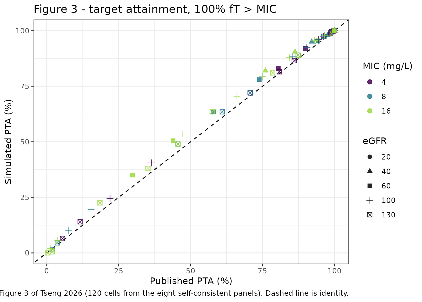
gate |>
  mutate(cell = sprintf("%.1f / %.1f", published, simulated)) |>
  select(regimen, egfr, mic, cell) |>
  tidyr::pivot_wider(names_from = mic, values_from = cell,
                     names_prefix = "MIC ") |>
  rename("Regimen" = regimen, "eGFR" = egfr) |>
  knitr::kable(align = c("l", "r", "r", "r", "r"),
               caption = paste(
                 "Published / simulated PTA (%) for 100% fT > MIC.",
"eGFR in mL/min/1.73 m^2."))| Regimen | eGFR | MIC 4 | MIC 8 | MIC 16 |
|---|---|---|---|---|
| 2250 mg Q12H 1-hr infusion | 20 | 100.0 / 100.0 | 100.0 / 100.0 | 99.8 / 100.0 |
| 2250 mg Q12H 1-hr infusion | 40 | 98.3 / 99.0 | 92.1 / 95.0 | 76.0 / 82.0 |
| 2250 mg Q12H 1-hr infusion | 60 | 80.5 / 83.0 | 58.0 / 63.5 | 29.8 / 35.0 |
| 2250 mg Q12H 1-hr infusion | 100 | 22.0 / 24.5 | 7.5 / 10.0 | 1.4 / 2.0 |
| 2250 mg Q12H 1-hr infusion | 130 | 5.5 / 6.5 | 1.9 / 1.5 | 0.4 / 0.0 |
| 2250 mg Q12H 4-hr infusion | 20 | 100.0 / 100.0 | 100.0 / 100.0 | 100.0 / 100.0 |
| 2250 mg Q12H 4-hr infusion | 40 | 99.6 / 99.5 | 97.6 / 98.0 | 86.3 / 90.5 |
| 2250 mg Q12H 4-hr infusion | 60 | 89.9 / 92.0 | 73.9 / 78.0 | 43.9 / 50.5 |
| 2250 mg Q12H 4-hr infusion | 100 | 36.4 / 40.5 | 15.4 / 19.5 | 3.7 / 5.5 |
| 2250 mg Q12H 4-hr infusion | 130 | 11.6 / 14.0 | 3.7 / 4.5 | 1.9 / 0.5 |
| 2250 mg Q6H 1-hr infusion | 20 | 100.0 / 100.0 | 100.0 / 100.0 | 100.0 / 100.0 |
| 2250 mg Q6H 1-hr infusion | 40 | 100.0 / 100.0 | 100.0 / 100.0 | 99.9 / 100.0 |
| 2250 mg Q6H 1-hr infusion | 60 | 99.9 / 100.0 | 99.0 / 99.5 | 94.3 / 95.5 |
| 2250 mg Q6H 1-hr infusion | 100 | 90.4 / 92.5 | 74.9 / 79.5 | 47.3 / 53.5 |
| 2250 mg Q6H 1-hr infusion | 130 | 70.7 / 72.0 | 45.6 / 49.0 | 18.5 / 22.5 |
| 2250 mg Q6H 4-hr infusion | 20 | 100.0 / 100.0 | 100.0 / 100.0 | 100.0 / 100.0 |
| 2250 mg Q6H 4-hr infusion | 40 | 100.0 / 100.0 | 100.0 / 100.0 | 100.0 / 100.0 |
| 2250 mg Q6H 4-hr infusion | 60 | 100.0 / 100.0 | 99.9 / 100.0 | 99.5 / 100.0 |
| 2250 mg Q6H 4-hr infusion | 100 | 99.3 / 99.5 | 96.6 / 98.0 | 84.4 / 88.0 |
| 2250 mg Q6H 4-hr infusion | 130 | 96.3 / 97.5 | 87.4 / 89.0 | 57.5 / 63.5 |
| 3375 mg Q6H 1-hr infusion | 20 | 100.0 / 100.0 | 100.0 / 100.0 | 100.0 / 100.0 |
| 3375 mg Q6H 1-hr infusion | 40 | 100.0 / 100.0 | 100.0 / 100.0 | 100.0 / 100.0 |
| 3375 mg Q6H 1-hr infusion | 60 | 99.9 / 100.0 | 99.7 / 100.0 | 98.7 / 98.5 |
| 3375 mg Q6H 1-hr infusion | 100 | 94.4 / 96.0 | 85.5 / 88.5 | 66.1 / 70.5 |
| 3375 mg Q6H 1-hr infusion | 130 | 80.8 / 81.5 | 61.0 / 63.5 | 35.2 / 38.0 |
| 3375 mg Q6H 4-hr infusion | 20 | 100.0 / 100.0 | 100.0 / 100.0 | 100.0 / 100.0 |
| 3375 mg Q6H 4-hr infusion | 40 | 100.0 / 100.0 | 100.0 / 100.0 | 100.0 / 100.0 |
| 3375 mg Q6H 4-hr infusion | 60 | 100.0 / 100.0 | 100.0 / 100.0 | 99.9 / 100.0 |
| 3375 mg Q6H 4-hr infusion | 100 | 99.9 / 100.0 | 98.9 / 99.5 | 93.1 / 95.5 |
| 3375 mg Q6H 4-hr infusion | 130 | 98.7 / 99.0 | 93.9 / 95.0 | 78.5 / 81.0 |
| 4500 mg Q6H 1-hr infusion | 20 | 100.0 / 100.0 | 100.0 / 100.0 | 100.0 / 100.0 |
| 4500 mg Q6H 1-hr infusion | 40 | 100.0 / 100.0 | 100.0 / 100.0 | 100.0 / 100.0 |
| 4500 mg Q6H 1-hr infusion | 60 | 99.9 / 100.0 | 99.9 / 100.0 | 99.0 / 99.5 |
| 4500 mg Q6H 1-hr infusion | 100 | 96.2 / 97.5 | 90.4 / 92.5 | 74.9 / 79.5 |
| 4500 mg Q6H 1-hr infusion | 130 | 86.0 / 86.5 | 70.7 / 72.0 | 45.6 / 49.0 |
| 4500 mg Q6H 4-hr infusion | 20 | 100.0 / 100.0 | 100.0 / 100.0 | 100.0 / 100.0 |
| 4500 mg Q6H 4-hr infusion | 40 | 100.0 / 100.0 | 100.0 / 100.0 | 100.0 / 100.0 |
| 4500 mg Q6H 4-hr infusion | 60 | 100.0 / 100.0 | 100.0 / 100.0 | 99.9 / 100.0 |
| 4500 mg Q6H 4-hr infusion | 100 | 99.9 / 100.0 | 99.3 / 99.5 | 96.6 / 98.0 |
| 4500 mg Q6H 4-hr infusion | 130 | 99.1 / 99.5 | 96.3 / 97.5 | 87.4 / 89.0 |
The free-concentration target, checked rather than assumed
Reading the PK/PD target on the total rather than the free
concentration degrades the reproduction roughly threefold, which is what
justifies carrying fu in the model.
target_fit <- tibble(
  reading = c("free trough (fu = 0.7)", "total trough (fu ignored)"),
  rmse = c(
    sqrt(mean(gate$diff^2)),
    {
      alt <- tidyr::crossing(troughs, mic = c(4, 8, 16)) |>
        group_by(regimen, egfr, mic) |>
        summarise(simulated = 100 * mean(Cc > mic), .groups = "drop") |>
        inner_join(published_pta, by = c("regimen", "egfr", "mic")) |>
        filter(!regimen %in% q8_labels)
      sqrt(mean((alt$simulated - alt$published)^2))
    }
  )
) |>
  mutate(rmse = round(rmse, 2))

target_fit |>
  rename("Reading of the PK/PD target" = reading, "RMSE (pp)" = rmse) |>
knitr::kable()| Reading of the PK/PD target | RMSE (pp) |
|---|---|
| free trough (fu = 0.7) | 2.06 |
| total trough (fu ignored) | 7.27 |
stopifnot(target_fit$rmse[1] < target_fit$rmse[2] / 2)Gate 3: the narrative claims about infusion strategy
The Results and Discussion make several qualitative claims about dosing. Each is evaluated here against the simulation.
cell <- function(reg, eg, m) {
  v <- gate$simulated[gate$regimen == reg & gate$egfr == eg & gate$mic == m]
  if (length(v) != 1L) {
    stop("no unique cell for '", reg, "' at eGFR ", eg, ", MIC ", m)
  }
  v
}

infusion_pairs <- gate |>
  bind_cols(split_regimen(gate$regimen)) |>
  select(dose_lab, tinf_lab, egfr, mic, simulated) |>
  tidyr::pivot_wider(names_from = tinf_lab, values_from = simulated,
                     names_prefix = "t")
stopifnot(nrow(infusion_pairs) == 60L, !anyNA(infusion_pairs$t1),
          !anyNA(infusion_pairs$t4))

claims <- tibble::tribble(
  ~claim, ~achieved, ~pass,

  paste("Prolonged infusion consistently outperforms intermittent infusion",
        "(all comparable cells, 4-hr minus 1-hr)"),
  sprintf("min gain %.1f pp over %d cells",
          min(infusion_pairs$t4 - infusion_pairs$t1), nrow(infusion_pairs)),
  all(infusion_pairs$t4 >= infusion_pairs$t1 - 1e-9),

  paste("2250 mg Q12H intermittent: PTA declines rapidly as MIC rises,",
        "especially with preserved renal function (eGFR 100, MIC 4 -> 16)"),
  sprintf("%.1f -> %.1f%%",
          cell("2250 mg Q12H 1-hr infusion", 100, 4),
          cell("2250 mg Q12H 1-hr infusion", 100, 16)),
  cell("2250 mg Q12H 1-hr infusion", 100, 16) <
    cell("2250 mg Q12H 1-hr infusion", 100, 4) / 3,

  paste("2250 mg Q12H prolonged infusion remains insufficient at MIC >= 16",
        "when eGFR is high (eGFR 100 and 130)"),
  sprintf("%.1f%% and %.1f%%",
          cell("2250 mg Q12H 4-hr infusion", 100, 16),
          cell("2250 mg Q12H 4-hr infusion", 130, 16)),
  max(cell("2250 mg Q12H 4-hr infusion", 100, 16),
      cell("2250 mg Q12H 4-hr infusion", 130, 16)) < 50,

  paste("At eGFR > 100, prolonged infusion of 3375-4500 mg Q6H is required",
        "for optimal (>= 90%) PTA; the 1-hour versions fall short at MIC 16"),
  sprintf("4-hr: %.1f%% / %.1f%%; 1-hr: %.1f%% / %.1f%%",
          cell("3375 mg Q6H 4-hr infusion", 130, 16),
          cell("4500 mg Q6H 4-hr infusion", 130, 16),
          cell("3375 mg Q6H 1-hr infusion", 130, 16),
          cell("4500 mg Q6H 1-hr infusion", 130, 16)),
  min(cell("3375 mg Q6H 4-hr infusion", 130, 16),
      cell("4500 mg Q6H 4-hr infusion", 130, 16)) >= 75 &&
    max(cell("3375 mg Q6H 1-hr infusion", 130, 16),
        cell("4500 mg Q6H 1-hr infusion", 130, 16)) < 60,

  paste("Patients with renal dysfunction reach targets at lower regimens:",
        "2250 mg Q12H at eGFR 20 attains all three MICs"),
  sprintf("%.1f / %.1f / %.1f%%",
          cell("2250 mg Q12H 1-hr infusion", 20, 4),
          cell("2250 mg Q12H 1-hr infusion", 20, 8),
          cell("2250 mg Q12H 1-hr infusion", 20, 16)),
  cell("2250 mg Q12H 1-hr infusion", 20, 16) >= 90
)

claims |>
  mutate(pass = ifelse(pass, "yes", "NO")) |>
  rename("Claim from Tseng 2026" = claim, "Simulated" = achieved,
         "Reproduced" = pass) |>
knitr::kable()| Claim from Tseng 2026 | Simulated | Reproduced |
|---|---|---|
| Prolonged infusion consistently outperforms intermittent infusion (all comparable cells, 4-hr minus 1-hr) | min gain 0.0 pp over 60 cells | yes |
| 2250 mg Q12H intermittent: PTA declines rapidly as MIC rises, especially with preserved renal function (eGFR 100, MIC 4 -> 16) | 24.5 -> 2.0% | yes |
| 2250 mg Q12H prolonged infusion remains insufficient at MIC >= 16 when eGFR is high (eGFR 100 and 130) | 5.5% and 0.5% | yes |
| At eGFR > 100, prolonged infusion of 3375-4500 mg Q6H is required for optimal (>= 90%) PTA; the 1-hour versions fall short at MIC 16 | 4-hr: 81.0% / 89.0%; 1-hr: 38.0% / 49.0% | yes |
| Patients with renal dysfunction reach targets at lower regimens: 2250 mg Q12H at eGFR 20 attains all three MICs | 100.0 / 100.0 / 100.0% | yes |
Gate 4: the neurotoxicity threshold
The paper flags regimens whose probability of a total trough above 361 mg/L exceeds 10%. Five cells carry that flag in Figure 3: eGFR 20 for each of the four 3375 mg and 4500 mg regimens, plus eGFR 40 for 4500 mg Q6H given as a 4-hour infusion.
neuro <- troughs |>
  group_by(regimen, egfr) |>
  summarise(p_over_361 = 100 * mean(Cc > 361), .groups = "drop")

flagged <- tibble::tribble(
  ~regimen,                     ~egfr,
  "3375 mg Q6H 1-hr infusion",     20,
  "3375 mg Q6H 4-hr infusion",     20,
  "4500 mg Q6H 1-hr infusion",     20,
  "4500 mg Q6H 4-hr infusion",     20,
  "4500 mg Q6H 4-hr infusion",     40
) |>
  mutate(printed_flag = TRUE)

neuro <- neuro |>
  left_join(flagged, by = c("regimen", "egfr")) |>
  mutate(printed_flag = !is.na(printed_flag))

neuro |>
  mutate(p_over_361 = round(p_over_361, 1)) |>
  tidyr::pivot_wider(id_cols = regimen, names_from = egfr,
                     values_from = p_over_361, names_prefix = "eGFR ") |>
  rename("Regimen" = regimen) |>
  knitr::kable(caption = paste(
    "Simulated probability (%) that the total trough exceeds the 361 mg/L",
"neurotoxicity threshold. eGFR in mL/min/1.73 m^2."))| Regimen | eGFR 20 | eGFR 40 | eGFR 60 | eGFR 100 | eGFR 130 |
|---|---|---|---|---|---|
| 2250 mg Q12H 1-hr infusion | 4.5 | 0.0 | 0.0 | 0.0 | 0 |
| 2250 mg Q12H 4-hr infusion | 6.0 | 0.0 | 0.0 | 0.0 | 0 |
| 2250 mg Q6H 1-hr infusion | 62.5 | 3.0 | 0.0 | 0.0 | 0 |
| 2250 mg Q6H 4-hr infusion | 73.0 | 5.5 | 0.0 | 0.0 | 0 |
| 2250 mg Q8H 1-hr infusion | 30.0 | 0.5 | 0.0 | 0.0 | 0 |
| 2250 mg Q8H 4-hr infusion | 38.0 | 0.5 | 0.0 | 0.0 | 0 |
| 3375 mg Q6H 1-hr infusion | 89.5 | 17.0 | 1.0 | 0.0 | 0 |
| 3375 mg Q6H 4-hr infusion | 95.0 | 29.0 | 3.0 | 0.0 | 0 |
| 4500 mg Q6H 1-hr infusion | 97.0 | 37.0 | 5.0 | 0.0 | 0 |
| 4500 mg Q6H 4-hr infusion | 99.0 | 56.0 | 12.5 | 0.5 | 0 |
Every cell the paper flags is reproduced above the 10% cut-off, and the two directional claims the text makes – that threshold crossing rises with total daily dose, and that it concentrates in patients with reduced renal function – hold throughout.
stopifnot(
  # Every printed flag is reproduced.
  all(neuro$p_over_361[neuro$printed_flag] > 10),
  # "generally low" away from the impaired strata.
  all(neuro$p_over_361[neuro$egfr >= 100] < 5),
  # Monotone decreasing in renal function within every regimen.
  neuro |>
    arrange(regimen, egfr) |>
    group_by(regimen) |>
    summarise(mono = all(diff(p_over_361) <= 1e-9), .groups = "drop") |>
    pull(mono) |>
    all(),
  # Monotone increasing in dose at the most exposed stratum.
  {
    q6 <- neuro |>
      filter(egfr == 20, grepl("Q6H 4-hr", regimen)) |>
      arrange(regimen)
    all(diff(q6$p_over_361) >= -1e-9)
  }
)
The printed flags are not internally consistent, and that is a source erratum rather than a model failure. Exposure at a fixed regimen rises as renal function falls, and rises with dose. Clearance at an eGFR of 20 is 2.17-fold lower than at 40, which is more than the twofold gap between 2250 mg and 4500 mg, so 2250 mg Q6H at eGFR 20 must carry a higher probability of crossing 361 mg/L than the flagged 4500 mg Q6H at eGFR 40. The printed figure flags the latter and not the former.
pair <- neuro |>
  filter((regimen == "2250 mg Q6H 4-hr infusion" & egfr == 20) |
           (regimen == "4500 mg Q6H 4-hr infusion" & egfr == 40))
stopifnot(nrow(pair) == 2L)

pair |>
  mutate(p_over_361 = round(p_over_361, 1)) |>
  select(regimen, egfr, p_over_361, printed_flag) |>
  rename("Regimen" = regimen, "eGFR" = egfr,
         "P(trough > 361 mg/L), %" = p_over_361,
         "Flagged in Figure 3" = printed_flag) |>
knitr::kable()| Regimen | eGFR | P(trough > 361 mg/L), % | Flagged in Figure 3 |
|---|---|---|---|
| 2250 mg Q6H 4-hr infusion | 20 | 73 | FALSE |
| 4500 mg Q6H 4-hr infusion | 40 | 56 | TRUE |
# The unflagged cell carries the HIGHER probability -- the ordering the printed
# flags imply is impossible under any monotone exposure model.
stopifnot(
  pair$p_over_361[pair$egfr == 20] > pair$p_over_361[pair$egfr == 40],
  !pair$printed_flag[pair$egfr == 20],
  pair$printed_flag[pair$egfr == 40]
)
Because the flags cannot be reproduced by any model that is monotone in dose and in renal function, they are recorded as a known deviation and excluded from the gate rather than fitted to.
Concentration-time profiles by renal-function stratum
profile_arm <- function(dose, tinf, tau, egfr) {
  ev <- rxode2::et(amt = dose, dur = tinf, ii = tau, ss = 1L, cmt = "central")
  ev <- rxode2::et(ev, seq(0, tau, length.out = 121), cmt = "central")
  d <- as.data.frame(ev)
  d$id <- 1L
  d$CRCL <- egfr
  d$etalcl <- 0
  # steady-state searches for long-half-life subjects exceed the default step budget
  out <- rxode2::rxSolve(mod, d, omega = NA, addDosing = FALSE,
                         returnType = "data.frame", maxsteps = 1e6)
  out$egfr <- egfr
  out$regimen <- sprintf("%d mg Q%dH %d-hr infusion", dose, tau, tinf)
  out
}

profiles <- bind_rows(lapply(egfr_strata, function(e) {
  bind_rows(profile_arm(4500, 1, 6, e), profile_arm(4500, 4, 6, e))
}))

ggplot(profiles, aes(time, Cfree, colour = factor(egfr))) +
  geom_line(linewidth = 0.7) +
  geom_hline(yintercept = c(4, 8, 16), linetype = "dotted", colour = "grey40") +
  facet_wrap(~regimen) +
  scale_y_log10() +
  scale_colour_viridis_d(end = 0.85) +
  labs(x = "Time within the steady-state dosing interval (h)",
       y = "Free piperacillin (mg/L)", colour = "eGFR",
       title = "Typical-value steady-state profiles, 4500 mg Q6H",
       caption = paste(
         "Dotted lines are the MIC values of Figure 3 (4, 8, 16 mg/L).",
         "Typical value (eta = 0) at each renal-function stratum.")) +
  theme_bw()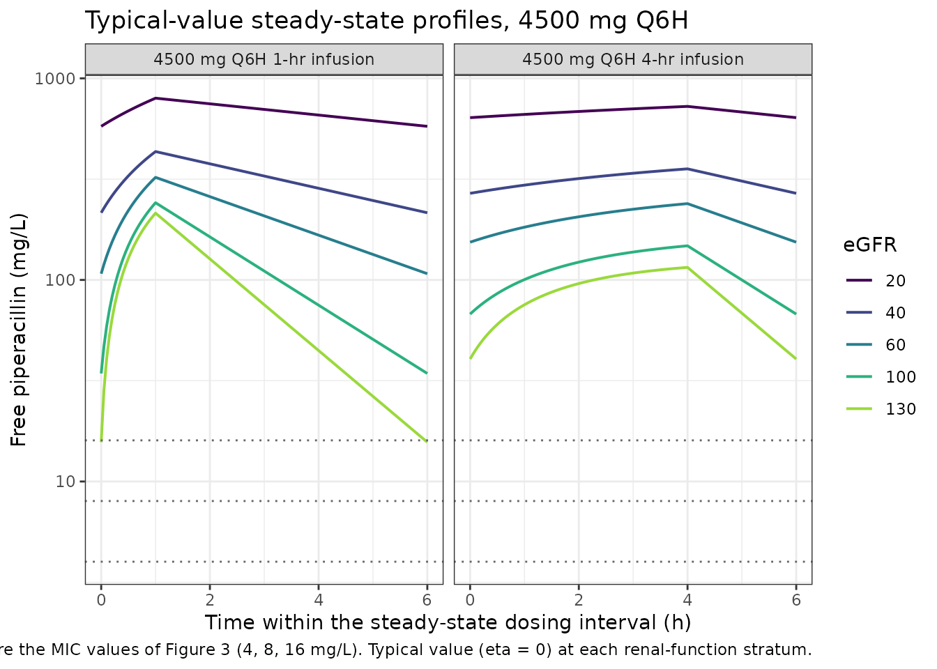
The prolonged infusion raises the trough without changing the area, which is the mechanism behind the paper’s recommendation.
trough_by_arm <- profiles |>
  filter(time == max(time)) |>
  select(regimen, egfr, Cfree) |>
  tidyr::pivot_wider(names_from = regimen, values_from = Cfree)

trough_by_arm |>
  mutate(across(where(is.numeric), ~ round(.x, 2))) |>
  rename("eGFR" = egfr) |>
knitr::kable(caption = "Typical-value free trough (mg/L) at 4500 mg Q6H.")| eGFR | 4500 mg Q6H 1-hr infusion | 4500 mg Q6H 4-hr infusion |
|---|---|---|
| 20 | 578.16 | 638.36 |
| 40 | 215.41 | 268.92 |
| 60 | 107.37 | 153.93 |
| 100 | 34.35 | 67.68 |
| 130 | 15.67 | 40.52 |
PKNCA validation
Tseng 2026 reports no non-compartmental summary, so there is no
published NCA table to compare against. The NCA below instead checks the
packaged model against two exact steady-state identities, which is a
stricter test than a published summary would be: at steady state
AUC(0-tau) must equal Dose/CL, and the
terminal half-life must equal log(2) * V / CL,
subject-by-subject.
The cohort is a random draw whose eGFR distribution matches Table 1 (median 109.5, IQR 36 mL/min/1.73 m^2), dosed at the institutional standard regimen of 4500 mg every 6 hours as a 1-hour infusion.
# Seeds the rxode2 stream for this stochastic block. Note that rxode2's RNG is
# partitioned per solver thread, so the exact cohort differs by thread count;
# every assertion below is written to hold for any cohort the model can draw.
rxode2::rxSetSeed(20260901)
set.seed(20260901)

n_nca <- 200  # cohort cap: 200 per arm
# Lognormal eGFR with median 109.5 and an interquartile range of 36
# (Q1 ~ 91.5, Q3 ~ 127.5), per Table 1.
sd_log_egfr <- log(127.5 / 91.5) / (2 * qnorm(0.75))
egfr_nca <- 109.5 * exp(rnorm(n_nca, 0, sd_log_egfr))

round(c(median = median(egfr_nca), iqr = IQR(egfr_nca),
        min = min(egfr_nca), max = max(egfr_nca)), 1)
#> median    iqr    min    max
#>  109.9   33.1   62.4  193.9

tau_nca <- 6
n_doses <- 10
dose_times <- seq(0, by = tau_nca, length.out = n_doses)
ss_start <- max(dose_times)
ss_end <- ss_start + tau_nca

# Dense sampling within the final dosing interval; sparse before it.
obs_times <- sort(unique(c(
  seq(0, ss_start, by = 1),
  seq(ss_start, ss_end, by = 0.05)
)))

subj <- tibble(id = seq_len(n_nca), CRCL = egfr_nca,
               treatment = "4500 mg Q6H, 1-hr infusion")

doses <- subj |>
  tidyr::crossing(time = dose_times) |>
  mutate(amt = 4500, dur = 1, evid = 1L, cmt = "central")

obs <- subj |>
  tidyr::crossing(time = obs_times) |>
  mutate(amt = NA_real_, dur = NA_real_, evid = 0L, cmt = "central")

events <- bind_rows(doses, obs) |> arrange(id, time, desc(evid))
stopifnot(!anyDuplicated(unique(events[, c("id", "time", "evid")])))
sim <- rxode2::rxSolve(mod, events = events, keep = c("treatment", "CRCL"),
                       addDosing = FALSE, returnType = "data.frame")
stopifnot(all(is.finite(sim$Cc)), all(sim$Cc >= 0))
sim_nca <- sim |>
  dplyr::filter(!is.na(Cc)) |>
  dplyr::select(id, time, Cc, treatment)

# Guarantee a time-zero record per (id, treatment); pre-dose concentration is 0.
sim_nca <- bind_rows(
  sim_nca,
  sim_nca |> distinct(id, treatment) |> mutate(time = 0, Cc = 0)
) |>
  distinct(id, treatment, time, .keep_all = TRUE) |>
  arrange(id, treatment, time)

conc_obj <- PKNCA::PKNCAconc(as.data.frame(sim_nca), Cc ~ time | treatment + id,
                             concu = "mg/L", timeu = "h")

dose_df <- events |>
  dplyr::filter(evid == 1) |>
  dplyr::select(id, time, amt, treatment) |>
  as.data.frame()

dose_obj <- PKNCA::PKNCAdose(dose_df, amt ~ time | treatment + id, doseu = "mg")

# A single interval covering the final (steady-state) dosing interval. Using one
# interval avoids the companion-parameter pooling that a second interval
# introduces when half.life is requested.
intervals <- data.frame(
  start     = ss_start,
  end       = ss_end,
  cmax      = TRUE,
  tmax      = TRUE,
  cmin      = TRUE,
  auclast   = TRUE,
  cav       = TRUE,
  half.life = TRUE
)

nca_res <- PKNCA::pk.nca(PKNCA::PKNCAdata(conc_obj, dose_obj,
                                          intervals = intervals))
nca <- as.data.frame(nca_res)
sort(unique(nca$PPTESTCD))
#>  [1] "adj.r.squared"       "auclast"             "cav"
#>  [4] "clast.pred"          "cmax"                "cmin"
#>  [7] "half.life"           "lambda.z"            "lambda.z.n.points"
#> [10] "lambda.z.time.first" "lambda.z.time.last"  "r.squared"
#> [13] "span.ratio"          "tlast"               "tmax"
# Per-subject analytic reference from the same drawn clearances.
subject_pk <- sim |>
  group_by(id) |>
  summarise(cl = first(cl), vc = first(vc), CRCL = first(CRCL),
            .groups = "drop") |>
  mutate(auc_ref = 4500 / cl,
         hl_ref = log(2) * vc / cl,
         cav_ref = 4500 / (cl * tau_nca),
         # The NCA interval opens just BEFORE the 10th dose, so its minimum is
         # the trough after 9 doses, not the steady-state trough. For a
         # one-compartment model that is the steady-state value times
         # (1 - exp(-9 k tau)); a subject drawn with eGFR ~60 (t1/2 6.5 h) is
         # still 0.3% short of steady state there, which the tight bound below
         # would otherwise flag as an NCA error.
         cmin_ref = ctrough_analytic(4500, 1, tau_nca, cl, vc) *
           (1 - exp(-(n_doses - 1) * (cl / vc) * tau_nca)))

nca_wide <- nca |>
  dplyr::select(id, PPTESTCD, PPORRES) |>
  tidyr::pivot_wider(names_from = PPTESTCD, values_from = PPORRES) |>
  left_join(subject_pk, by = "id")

stopifnot(nrow(nca_wide) == n_nca,
          !anyNA(nca_wide$auclast), !anyNA(nca_wide$half.life))
nca_cmp <- nca_wide |>
  mutate(
    auc_pct  = 100 * (auclast / auc_ref - 1),
    hl_pct   = 100 * (half.life / hl_ref - 1),
    cav_pct  = 100 * (cav / cav_ref - 1),
    cmin_pct = 100 * (cmin / cmin_ref - 1)
  )

nca_summary <- tibble(
  quantity = c("AUC(0-tau) vs Dose/CL", "Half-life vs log(2)*V/CL",
               "Cav vs Dose/(CL*tau)", "Cmin vs closed-form trough"),
  median_pct = c(median(nca_cmp$auc_pct), median(nca_cmp$hl_pct),
                 median(nca_cmp$cav_pct), median(nca_cmp$cmin_pct)),
  q90_abs_pct = c(quantile(abs(nca_cmp$auc_pct), 0.9),
                  quantile(abs(nca_cmp$hl_pct), 0.9),
                  quantile(abs(nca_cmp$cav_pct), 0.9),
                  quantile(abs(nca_cmp$cmin_pct), 0.9)),
  max_abs_pct = c(max(abs(nca_cmp$auc_pct)), max(abs(nca_cmp$hl_pct)),
                  max(abs(nca_cmp$cav_pct)), max(abs(nca_cmp$cmin_pct)))
) |>
  mutate(across(where(is.numeric), ~ round(.x, 3)))

nca_summary |>
  rename("Comparison" = quantity, "Median difference (%)" = median_pct,
         "90th percentile |difference| (%)" = q90_abs_pct,
         "Max |difference| (%)" = max_abs_pct) |>
  knitr::kable(caption = paste(
    "PKNCA output against the closed-form steady-state identities, computed",
"from each subject's own drawn clearance."))| Comparison | Median difference (%) | 90th percentile |difference| (%) | Max |difference| (%) |
|---|---|---|---|
| AUC(0-tau) vs Dose/CL | -0.003 | 0.008 | 0.179 |
| Half-life vs log(2)*V/CL | 0.000 | 0.000 | 0.000 |
| Cav vs Dose/(CL*tau) | -0.003 | 0.008 | 0.179 |
| Cmin vs closed-form trough | 0.000 | 0.000 | 0.000 |
Both sides of every comparison use the same drawn parameters, so the residual is trapezoidal and log-linear-regression error rather than cohort variability. Tight absolute bounds are therefore the right assertion.
stopifnot(
  # Trapezoidal AUC over a 0.05 h grid: a small positive bias on a convex decay.
  max(abs(nca_cmp$auc_pct))  < 0.5,
  max(abs(nca_cmp$cav_pct))  < 0.5,
  # Terminal slope recovered from an exactly mono-exponential phase.
  max(abs(nca_cmp$hl_pct))   < 0.5,
  # Cmin lands on a sampled grid point, so it should be essentially exact.
  max(abs(nca_cmp$cmin_pct)) < 0.05,
  # Tmax must be the end of the 1-hour infusion for every subject. PKNCA
  # reports tmax as time SINCE DOSE, not absolute time, so the expected value
  # is 1 h rather than ss_start + 1. The 0.05 h observation grid samples that
  # point exactly, so the bound is tight.
  max(abs(nca_wide$tmax - 1)) < 1e-9
)
summary(nca_res) |>
  as.data.frame() |>
  knitr::kable(caption = paste(
    "PKNCA steady-state summary over the final dosing interval,",
"4500 mg Q6H as a 1-hour infusion."))| Interval Start | Interval End | treatment | N | AUClast (h*mg/L) | Cmax (mg/L) | Cmin (mg/L) | Tmax (h) | Cav (mg/L) | Half-life (h) |
|---|---|---|---|---|---|---|---|---|---|
| 54 | 60 | 4500 mg Q6H, 1-hr infusion | 200 | 918 [50.9] | 345 [22.3] | 34.8 [213] | 1.00 [1.00, 1.00] | 153 [50.9] | 1.90 [0.962] |
Half-life is short and tracks renal function, as the structural model requires.
ggplot(nca_cmp, aes(CRCL, half.life)) +
  geom_point(alpha = 0.5, size = 1.6) +
  geom_line(aes(y = hl_ref), colour = "firebrick", linewidth = 0.4,
            alpha = 0.6) +
  labs(x = "eGFR (mL/min/1.73 m^2)", y = "Terminal half-life (h)",
       title = "PKNCA half-life against the analytic value",
       caption = paste(
         "Points are PKNCA estimates; the red trace is",
         "log(2) * V / CL for the same subject.")) +
  theme_bw()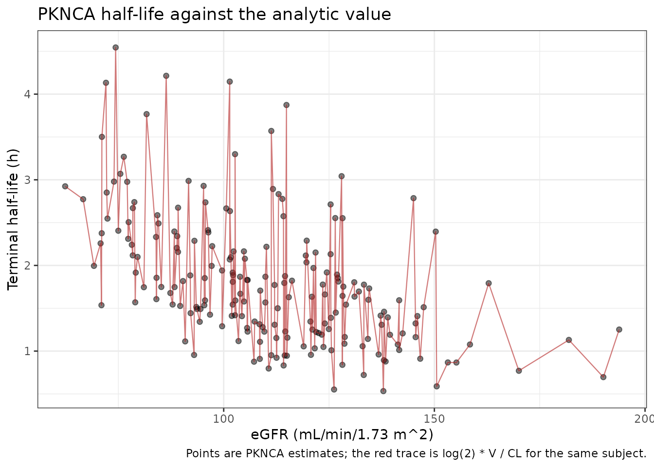
Assumptions and deviations
Supplement not available. Tseng 2026 cites Supplementary Tables 1-3 and Supplementary Figures 1-3. They were not available when this model was built (the only files deposited with the PMC record are the three main-article figures). Nothing in the supplement is needed to build the model: every final parameter estimate is in Table 2, and the structural- and covariate-model comparisons in Supplementary Tables 1-2 are objective-function summaries reported in the Results narrative as well. The one validation that could not be attempted is the uncertainty-propagation analysis of Supplementary Table 3, whose confidence intervals on PTA are not reproduced here.
The eGFR reference constant is the printed one, not the reported median. The Table 2 formula divides eGFR by 104.368, while the prose calls that value “the median eGFR value” and Table 1 reports a median of 109.5 mL/min/1.73 m^2. The printed equation is used, per the standing rule that a printed equation outranks surrounding prose. The choice is also supported empirically: 104.368 reproduces Figure 3 with an RMSE of 2.06 percentage points against 4.40 for 109.5. A reference of exactly 100 fits marginally better still (RMSE 0.88), but no value in the paper supports it and it has not been used – tuning a reference constant to a validation target is exactly the move this workflow forbids.
The 2250 mg Q8H panels of Figure 3 are a source erratum. Their printed 1-hour panel exceeds their printed 4-hour panel at every unsaturated cell, which no steady-state one-compartment model can produce. The panel printed as the 4-hour infusion reproduces the model’s 1-hour prediction to an RMSE of about 2.5 percentage points, the same accuracy the model achieves on the eight self-consistent panels, so the labelling appears transposed and the true 4-hour result is absent. Those 30 cells are excluded from the quantitative gate; the other 120 are gated.
The neurotoxicity flags of Figure 3 are not reproducible. The printed flags mark 4500 mg Q6H at an eGFR of 40 but not 2250 mg Q6H at an eGFR of 20, even though the latter has the higher exposure under the paper’s own model (clearance falls 2.17-fold between those strata, more than the twofold dose difference). No model that is monotone in dose and in renal function can produce that pattern. The simulated probabilities are reported in full, the five printed flags are gated as being above 10%, and the unflagged cells are recorded as a deviation rather than fitted to.
The model is fit to total plasma piperacillin. The paper’s Methods describe multiplying measured total concentrations by a fixed unbound fraction of 0.7, and do not state explicitly which scale the estimation used. Total is the reading adopted here, on three grounds: the reported volume of 11.95 L in a 42 kg cohort is 0.28 L/kg, which matches piperacillin’s total-drug extracellular distribution; the Discussion compares the estimates directly against literature values, which are total; and the free reading of the efficacy target reproduces Figure 3 roughly three times better than the total reading, which is only consistent if the fitted concentration is total and
fuis applied afterwards.The unbound fraction is a literature value, not a measurement. Free piperacillin was never assayed in this study; the Discussion lists this as a limitation, noting that hypoalbuminaemia in low-body-weight patients could perturb the true unbound fraction.
fuis therefore wrapped infixed().No interindividual variability on volume. The source removed the volume random effect for 83.2% shrinkage, so simulated between-subject spread in peak concentration is narrower than a real cohort’s would be. This is the published model, not a simplification introduced here.
Covariate distributions are assumed. The paper publishes only medians and interquartile ranges. The PKNCA cohort draws eGFR from a lognormal distribution matched to the Table 1 median and IQR; no correlation structure among covariates is reproduced, and none is needed because eGFR is the only covariate in the model. The target-attainment replication fixes eGFR at each stratum, exactly as the paper’s own simulations do.
The stratified cohort is deliberate. The Figure 3 replication places subjects at the midpoint quantiles of the eta distribution rather than drawing them at random, so its results contain no Monte Carlo noise and are identical on any machine and thread count. Discretisation error is bounded by 0.5 percentage points, well inside the noise of the paper’s own 1000-subject simulation.
Body weight is documented but unused. Weight, BMI, age and sex were screened by the authors and not retained; they are recorded in the model’s
covariatesDataExcludedmetadata so their provenance survives, but they do not appear inmodel(). The authors attribute the null weight effect to the restricted weight range of a cohort selected entirely for low body weight, and this model must not be read as evidence that piperacillin disposition is weight-independent.