Dabrafenib, hydroxy-dabrafenib and trametinib (Balakirouchenane 2020)
Source:vignettes/articles/Balakirouchenane_2020_dabrafenib_trametinib.Rmd
Balakirouchenane_2020_dabrafenib_trametinib.RmdModels and source
mod_dab <- rxode2::rxode(readModelDb("Balakirouchenane_2020_dabrafenib"))
#> ℹ parameter labels from comments will be replaced by 'label()'
#> Warning: some etas defaulted to non-mu referenced, possible parsing error: etaiov_cl_1, etaiov_cl_2, etaiov_cl_3, etaiov_cl_4, etaiov_cl_5, etaiov_cl_6
#> as a work-around try putting the mu-referenced expression on a simple line
mod_tra <- rxode2::rxode(readModelDb("Balakirouchenane_2020_trametinib"))
#> ℹ parameter labels from comments will be replaced by 'label()'- Citation: Balakirouchenane D, Guegan S, Csajka C, Jouinot A, Heidelberger V, Puszkiel A, Zehou O, Khoudour N, Courlet P, Kramkimel N, Lheure C, Franck N, Huillard O, Arrondeau J, Vidal M, Goldwasser F, Maubec E, Dupin N, Aractingi S, Guidi M, Blanchet B. Population Pharmacokinetics/Pharmacodynamics of Dabrafenib Plus Trametinib in Patients with BRAF-Mutated Metastatic Melanoma. Cancers. 2020;12(4):931. doi:10.3390/cancers12040931. Parameter estimates from Table 2 (final model column); the covariate equations from the Table 2 footnote; population from Table 1.
- Article: https://doi.org/10.3390/cancers12040931
Balakirouchenane and colleagues fit two population PK models to routine-care samples from French patients treated with the BRAF inhibitor dabrafenib, alone or combined with the MEK inhibitor trametinib, and then related the model-based exposures to dose-limiting toxicity and survival. The two PK models were fit separately and are shipped as two files that share this article:
-
Balakirouchenane_2020_dabrafenib– Joint parent-metabolite population PK model for oral dabrafenib and its active metabolite hydroxy-dabrafenib in a real-life cohort of adults with BRAF V600-mutated solid tumours, mostly metastatic melanoma (Balakirouchenane 2020). Dabrafenib is two-compartment with first-order absorption (rate constant fixed to a literature value) and an absorption lag time, and is eliminated exclusively by irreversible conversion to hydroxy-dabrafenib, which is itself two-compartment with first-order elimination. All disposition parameters are apparent oral values. Dabrafenib apparent clearance decreases linearly with age (median-centred at 61.2 years) and is 17% lower in women; hydroxy-dabrafenib apparent clearance decreases linearly with age. Inter-individual variability on dabrafenib CL/F and V2/F and on hydroxy-dabrafenib CLm/F and V3/F, inter-occasion variability on dabrafenib CL/F, and proportional residual error on both analytes. -
Balakirouchenane_2020_trametinib– Two-compartment population PK model with first-order absorption, an absorption lag time and linear elimination for oral trametinib in a real-life cohort of adults with BRAF V600-mutated solid tumours, mostly metastatic melanoma, co-treated with dabrafenib (Balakirouchenane 2020). All disposition parameters are apparent oral values. No covariate was retained. Inter-individual variability on CL/F and Q/F; additive residual error.
The exposure-response part of the paper (Fisher / Wilcoxon tests for dose-limiting toxicity, Cox models for overall and progression-free survival) is a statistical analysis of per-patient AUCs and has no structural model to encode.
Population
Seventy-three adults with BRAF V600-mutated metastatic solid tumours contributed 424 dabrafenib / hydroxy-dabrafenib records; the 60 who also took trametinib contributed 318 trametinib concentrations (Table 1). Most had metastatic melanoma (89% in the dabrafenib set, 87% in the trametinib set); the rest had anaplastic thyroid or non-small-cell lung carcinoma. In the dabrafenib set the median (range) age was 61.2 (20-90) years and body weight 73.0 (51.7-166.0) kg, and 41% were women; 78% took a proton-pump inhibitor. Patients started dabrafenib at 150 mg twice daily and trametinib at 2 mg once daily, with reduced starting doses allowed. All samples were drawn at steady state during routine visits at three Paris hospitals between July 2015 and June 2017.
str(mod_dab$population[c("n_subjects", "age_range", "sex_female_pct", "dose_range")])
#> List of 4
#>  $ n_subjects    : int 73
#>  $ age_range     : chr "20-90 years (median 61.2)"
#>  $ sex_female_pct: num 41
#>  $ dose_range    : chr "Dabrafenib 150 mg orally twice daily (reduced starting doses such as 75 mg twice daily allowed at physician dis"| __truncated__
Source trace
| Element | Value | Source |
|---|---|---|
| Dabrafenib / OHD structure: 2-cmt parent, lag + first-order absorption, complete conversion to 2-cmt metabolite | – | Results 2.2.1; Figure 1; Methods 4.4.1 |
lka (fixed) |
1.8 1/h | Table 2; Methods 4.4.1 |
ltlag |
0.499 h | Table 2 |
lcl, lvc, lq,
lvp
|
19.3 L/h, 39.1 L, 3.40 L/h, 18.7 L | Table 2 (CL/F, V2/F, Q/F, V4/F) |
lcl_ohdab, lvc_ohdab,
lq_ohdab, lvp_ohdab
|
23.2 L/h, 5.11 L, 7.21 L/h, 27.1 L | Table 2 (CLm/F, V3/F, Qm/F, V5/F) |
e_age_cl, e_age_cl_ohdab
|
-0.536, -0.589 | Table 2 (unsigned); sign from Results 2.2.1 and Figure 3 |
e_sexf_cl |
0.832 | Table 2 |
| Covariate equations, MAGE = 61.2 y, Sex 1 = woman | – | Table 2 footnote |
etalcl, etalvc, etalcl_ohdab,
etalvc_ohdab
|
16.0, 50.8, 24.0, 47.5 %CV | Table 2 |
etaiov_cl_* |
17.4 %CV | Table 2 ‘IOV’ |
propSd, propSd_ohdab
|
48.7%, 53.1% | Table 2 (correlation 87.0% not encoded) |
| Molecular weights 519.56 / 535.56 g/mol | – | Computed from the formulas; analysis in molar units per Methods 4.4 |
| Trametinib structure: 2-cmt, lag + first-order absorption | – | Results 2.2.2 |
lka, ltlag, lcl,
lvc, lq, lvp
|
0.913 1/h, 0.709 h, 5.83 L/h, 61.9 L, 64.9 L/h, 417.0 L | Table 3 |
etalcl, etalq
|
29.6, 80.2 %CV | Table 3 |
addSd |
4.14 ng/mL | Table 3 |
Typical-value check against Figure 3
Figure 3 of the paper simulates 150 mg dabrafenib twice daily in men and women aged 20 and 90 and reports the median composite AUC (dabrafenib + hydroxy-dabrafenib over one dosing interval). With IIV switched off the model should reproduce those medians, which makes this the most direct check of the age and sex covariate equations, including the sign of the age coefficients and the molar conversion from dabrafenib to hydroxy-dabrafenib.
groups <- tibble::tribble(
  ~group,         ~AGE, ~SEXF, ~published,
  "Men, 20 y",      20,     0,      10447,
  "Men, 90 y",      90,     0,      19542,
  "Women, 20 y",    20,     1,      11632,
  "Women, 90 y",    90,     1,      21707
)

tau <- 12
ss_start <- 29 * 24 + 12 # start of the 60th dosing interval

make_dab_events <- function(n_per_group, groups) {
  base <- rxode2::et(amt = 150, ii = tau, addl = 59, cmt = "depot") |>
    # dense over the lag time and absorption peak, where a coarse grid biases
    # the trapezoidal AUC
    rxode2::et(ss_start + c(seq(0, 3, by = 0.05), seq(3.25, tau, by = 0.25))) |>
    as.data.frame()
  out <- lapply(seq_len(nrow(groups)), function(i) {
    ids <- (i - 1) * n_per_group + seq_len(n_per_group)
    do.call(rbind, lapply(ids, function(j) {
      d <- base
      d$id <- j
      d
    })) |>
      dplyr::mutate(group = groups$group[i], AGE = groups$AGE[i], SEXF = groups$SEXF[i])
  })
  dplyr::bind_rows(out) |>
    dplyr::mutate(
      OCC = 1L,
      # Two declared endpoints, neither an ODE state: key observation rows by dvid
      dvid = ifelse(evid == 0, 1L, NA_integer_),
      cmt = ifelse(evid == 0, NA_character_, cmt)
    )
}

trap <- function(t, y) sum(diff(t) * (head(y, -1) + tail(y, -1)) / 2)

ev_typ <- make_dab_events(1, groups)
sim_typ <- as.data.frame(rxode2::rxSolve(mod_dab, ev_typ, omega = NA, sigma = NA,
                                         keep = "group"))

typ <- sim_typ |>
  dplyr::group_by(group) |>
  dplyr::summarise(auc_dab = trap(time, Cc), auc_ohdab = trap(time, Cc_ohdab), .groups = "drop") |>
  dplyr::mutate(composite = auc_dab + auc_ohdab) |>
  dplyr::left_join(groups, by = "group") |>
  dplyr::mutate(pct_diff = 100 * (composite - published) / published)

typ |>
  dplyr::select(group, auc_dab, auc_ohdab, composite, published, pct_diff) |>
  dplyr::mutate(dplyr::across(c(auc_dab, auc_ohdab, composite), round)) |>
  dplyr::rename(
    "Group" = group, "AUCtau DAB (ng.h/mL)" = auc_dab,
    "AUCtau OHD (ng.h/mL)" = auc_ohdab, "Composite (ng.h/mL)" = composite,
    "Figure 3 median (ng.h/mL)" = published, "% difference" = pct_diff
  ) |>
knitr::kable(digits = 2, caption = "Typical-value composite AUC vs Figure 3 medians.")| Group | AUCtau DAB (ng.h/mL) | AUCtau OHD (ng.h/mL) | Composite (ng.h/mL) | Figure 3 median (ng.h/mL) | % difference |
|---|---|---|---|---|---|
| Men, 20 y | 5713 | 4774 | 10487 | 10447 | 0.39 |
| Men, 90 y | 10395 | 9222 | 19617 | 19542 | 0.38 |
| Women, 20 y | 6866 | 4774 | 11640 | 11632 | 0.07 |
| Women, 90 y | 12494 | 9221 | 21715 | 21707 | 0.04 |
Stochastic steady-state simulation (dabrafenib / hydroxy-dabrafenib)
Two hundred virtual patients per Figure 3 group receive 150 mg twice daily for 30 days, one occasion each. The composite AUC distribution per group is the stochastic analogue of Figure 3.
rxode2::rxSetSeed(20200409)
n_per_group <- 200
ev_dab <- make_dab_events(n_per_group, groups)
sim_dab <- as.data.frame(rxode2::rxSolve(mod_dab, ev_dab, keep = "group",
                                         returnType = "data.frame"))
sim_dab |>
  dplyr::select(id, time, group, Cc, Cc_ohdab) |>
  tidyr::pivot_longer(c(Cc, Cc_ohdab), names_to = "analyte", values_to = "conc") |>
  dplyr::mutate(analyte = ifelse(analyte == "Cc", "Dabrafenib", "Hydroxy-dabrafenib"),
                tad = time - ss_start) |>
  dplyr::group_by(group, analyte, tad) |>
  dplyr::summarise(p05 = quantile(conc, 0.05), p50 = median(conc),
                   p95 = quantile(conc, 0.95), .groups = "drop") |>
  ggplot(aes(tad, p50, colour = group, fill = group)) +
  geom_ribbon(aes(ymin = p05, ymax = p95), alpha = 0.15, colour = NA) +
  geom_line() +
  facet_wrap(~analyte) +
  labs(x = "Time after dose (h)", y = "Concentration (ng/mL)", colour = NULL, fill = NULL) +
  theme_bw()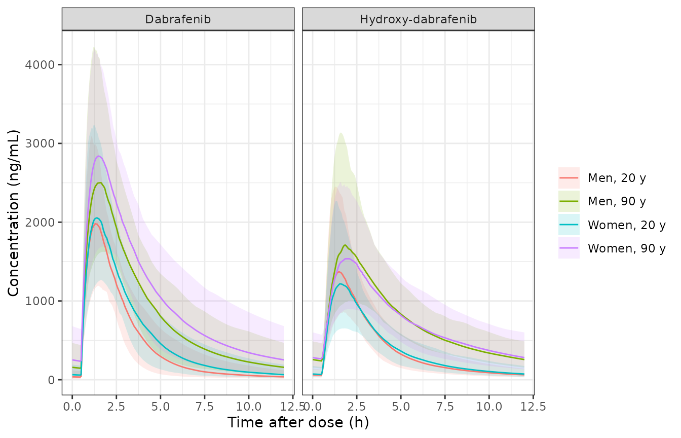
Steady-state profiles over one 12-h interval: median and 5th-95th percentiles of the individual predictions (no residual error), by Figure 3 group. The shape corresponds to the pcVPC of Figure 2.
PKNCA over the steady-state interval
nca_in <- sim_dab |>
  dplyr::select(id, time, group, Cc, Cc_ohdab) |>
  tidyr::pivot_longer(c(Cc, Cc_ohdab), names_to = "analyte", values_to = "conc") |>
  dplyr::filter(!is.na(conc)) |>
  dplyr::rename(treatment = group)

dose_dab <- ev_dab |>
  dplyr::filter(evid == 1) |>
  dplyr::transmute(id, time, amt, treatment = group)

conc_obj <- PKNCA::PKNCAconc(nca_in, conc ~ time | treatment + id / analyte)
dose_obj <- PKNCA::PKNCAdose(dose_dab, amt ~ time | treatment + id)
intervals <- data.frame(start = ss_start, end = ss_start + tau,
                        auclast = TRUE, cmax = TRUE, cmin = TRUE, tmax = TRUE)
nca_dab <- PKNCA::pk.nca(PKNCA::PKNCAdata(conc_obj, dose_obj, intervals = intervals))

nca_wide <- as.data.frame(nca_dab) |>
  dplyr::select(treatment, id, analyte, PPTESTCD, PPORRES) |>
  tidyr::pivot_wider(names_from = c(analyte, PPTESTCD), values_from = PPORRES)
stopifnot(nrow(nca_wide) == 4 * n_per_group)
Internal identity: steady-state AUCtau equals Dose / CL
At steady state the dabrafenib AUC over a dosing interval is exactly
Dose / CL, and, because conversion to the metabolite is
complete, the hydroxy-dabrafenib AUC is Dose / CLm scaled
by the molecular-weight ratio. Both sides use each subject’s own drawn
parameters, so the difference is pure trapezoidal error and a tight
bound is appropriate.
indiv <- sim_dab |>
  dplyr::distinct(id, cl, cl_ohdab)
ident <- nca_wide |>
  dplyr::left_join(indiv, by = "id") |>
  dplyr::mutate(
    dab_pct = 100 * (Cc_auclast - 150 / cl * 1000) / (150 / cl * 1000),
    ohdab_ref = 150 / cl_ohdab * (535.56 / 519.56) * 1000,
    ohdab_pct = 100 * (Cc_ohdab_auclast - ohdab_ref) / ohdab_ref
  )
knitr::kable(tibble::tibble(
  Analyte = c("Dabrafenib", "Hydroxy-dabrafenib"),
  "Max absolute % difference" = c(max(abs(ident$dab_pct)), max(abs(ident$ohdab_pct)))
), digits = 3, caption = "PKNCA AUCtau vs the analytic steady-state value.")| Analyte | Max absolute % difference |
|---|---|
| Dabrafenib | 0.093 |
| Hydroxy-dabrafenib | 0.019 |
Comparison against Figure 3
sim_summary <- nca_wide |>
  dplyr::mutate(composite = Cc_auclast + Cc_ohdab_auclast) |>
  dplyr::group_by(treatment) |>
  dplyr::summarise(auclast = median(composite), .groups = "drop")

published <- groups |>
  dplyr::transmute(treatment = group, auclast = published)

cmp <- nlmixr2lib::ncaComparisonTable(
  simulated = sim_summary,
  reference = published,
  by = "treatment",
  params = "auclast",
  units = c(auclast = "ng.h/mL"),
  tolerance_pct = 20
)
knitr::kable(cmp, caption = paste(
  "Median composite AUCtau (dabrafenib + hydroxy-dabrafenib) of 200 simulated",
  "patients per group vs the Figure 3 medians. * differs by >20%."
))| NCA parameter | treatment | Reference | Simulated | % diff |
|---|---|---|---|---|
| AUClast (ng.h/mL) | Men, 20 y | 10400 | 10500 | +0.8% |
| AUClast (ng.h/mL) | Men, 90 y | 19500 | 19400 | -0.7% |
| AUClast (ng.h/mL) | Women, 20 y | 11600 | 11700 | +0.4% |
| AUClast (ng.h/mL) | Women, 90 y | 21700 | 21700 | -0.1% |
chk <- sim_summary |>
  dplyr::left_join(published, by = "treatment", suffix = c("_sim", "_pub")) |>
  dplyr::mutate(pct = 100 * (auclast_sim - auclast_pub) / auclast_pub)
# Median of 200 log-normal draws with ~20-30% CV: Monte-Carlo error ~2%.
stopifnot(all(abs(chk$pct) < 7))
The paper’s Section 2.4 also reports the median model-estimated AUC over the first three months in the 30 melanoma patients of the survival analysis: 7722 ng.h/mL for dabrafenib and 6082 ng.h/mL for hydroxy-dabrafenib, a hydroxy-dabrafenib / dabrafenib ratio near the 0.80 the Discussion quotes. Those are empirical Bayes estimates in a cohort that included reduced doses, so they are context rather than a gate; the simulated 150 mg values at the cohort’s median age are of the same order.
ev_med <- make_dab_events(1, tibble::tibble(group = "Man, 61.2 y", AGE = 61.2, SEXF = 0))
sim_med <- as.data.frame(rxode2::rxSolve(mod_dab, ev_med, omega = NA, sigma = NA))
c(auc_dab = trap(sim_med$time, sim_med$Cc), auc_ohdab = trap(sim_med$time, sim_med$Cc_ohdab))
#>   auc_dab auc_ohdab
#>  7773.870  6666.561
Trametinib
rxode2::rxSetSeed(20200410)
n_tra <- 200
# 60 days: with IIV of 80% on Q/F and a 417 L peripheral volume, subjects with
# a low Q/F take several weeks to approach steady state.
ss_tra <- 59 * 24
ev_tra <- rxode2::et(amt = 2, ii = 24, addl = 59, cmt = "depot") |>
  rxode2::et(ss_tra + c(seq(0, 4, by = 0.05), seq(4.25, 24, by = 0.25)), cmt = "central") |>
  rxode2::et(id = seq_len(n_tra)) |>
  as.data.frame() |>
  dplyr::mutate(treatment = "2 mg once daily")
sim_tra <- as.data.frame(rxode2::rxSolve(mod_tra, ev_tra, keep = "treatment",
                                         returnType = "data.frame"))
sim_tra |>
  dplyr::mutate(tad = time - ss_tra) |>
  dplyr::group_by(tad) |>
  dplyr::summarise(p05 = quantile(Cc, 0.05), p50 = median(Cc), p95 = quantile(Cc, 0.95)) |>
  ggplot(aes(tad, p50)) +
  geom_ribbon(aes(ymin = p05, ymax = p95), alpha = 0.2) +
  geom_line() +
  labs(x = "Time after dose (h)", y = "Trametinib (ng/mL)") +
  theme_bw()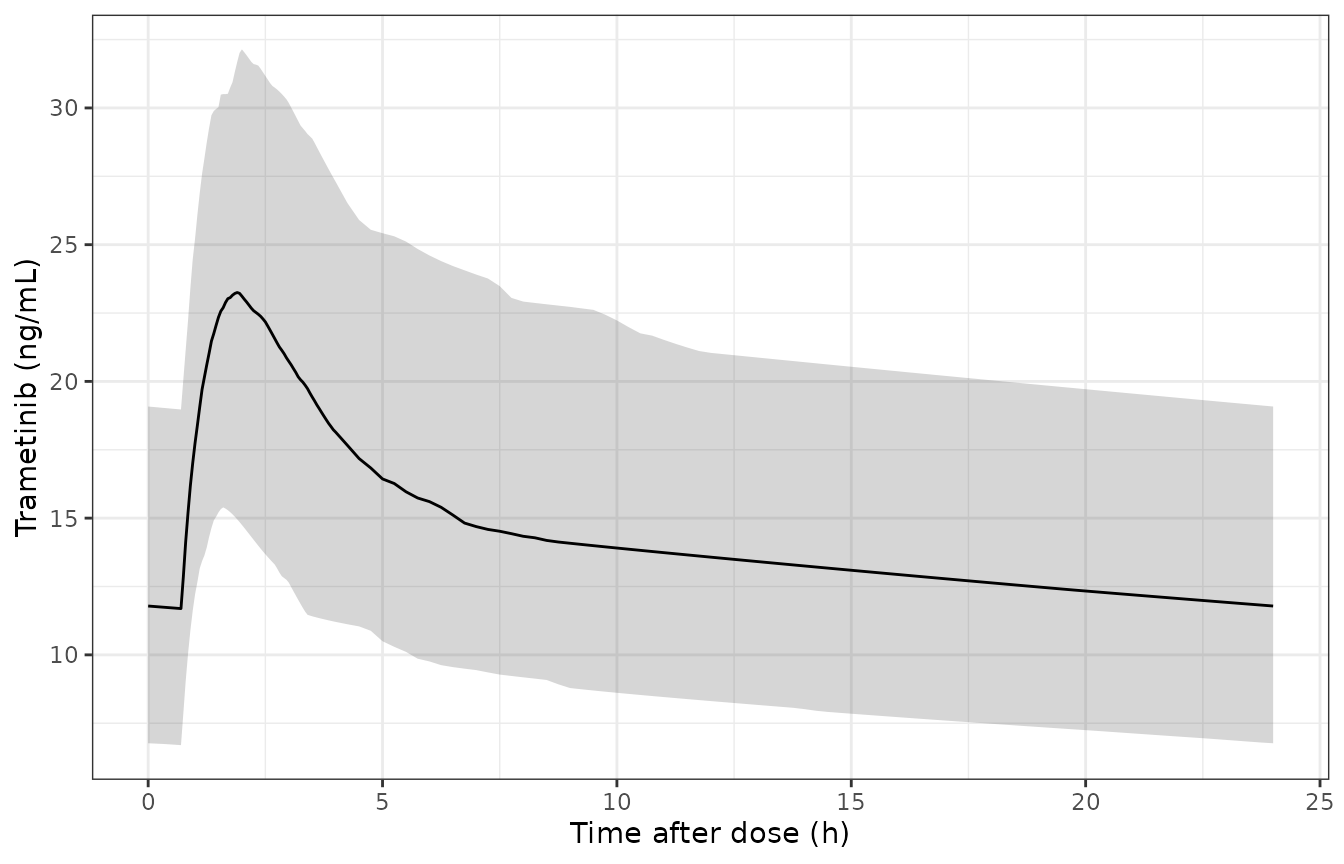
Trametinib steady-state profile over one 24-h interval: median and 5th-95th percentiles of the individual predictions (compare Figure 4).
conc_tra <- PKNCA::PKNCAconc(
  sim_tra |> dplyr::filter(!is.na(Cc)) |> dplyr::select(id, time, Cc, treatment),
  Cc ~ time | treatment + id
)
dose_tra <- PKNCA::PKNCAdose(
  ev_tra |> dplyr::filter(evid == 1) |> dplyr::select(id, time, amt, treatment),
  amt ~ time | treatment + id
)
int_tra <- data.frame(start = ss_tra, end = ss_tra + 24,
                      auclast = TRUE, cmax = TRUE, cmin = TRUE, tmax = TRUE)
nca_tra <- PKNCA::pk.nca(PKNCA::PKNCAdata(conc_tra, dose_tra, intervals = int_tra))
tra_wide <- as.data.frame(nca_tra) |>
  tidyr::pivot_wider(id_cols = c(treatment, id), names_from = PPTESTCD, values_from = PPORRES) |>
  dplyr::left_join(sim_tra |> dplyr::distinct(id, cl), by = "id") |>
  dplyr::mutate(pct = 100 * (auclast - 2 / cl * 1000) / (2 / cl * 1000))
# Dose / CL holds only at true steady state; the residual gap is the slow
# peripheral approach in low-Q/F subjects (a per-subject physical effect), so
# gate on the centre and a robust quantile rather than on the maximum.
stopifnot(
  nrow(tra_wide) == n_tra,
  abs(median(tra_wide$pct)) < 0.5,
  quantile(abs(tra_wide$pct), 0.9) < 1
)

tra_summary <- tra_wide |>
  dplyr::group_by(treatment) |>
  dplyr::summarise(auclast = median(auclast), cmax = median(cmax),
                   cmin = median(cmin), .groups = "drop")
tra_pub <- tibble::tibble(treatment = "2 mg once daily", auclast = 292)

knitr::kable(nlmixr2lib::ncaComparisonTable(
  simulated = tra_summary, reference = tra_pub, by = "treatment",
  params = "auclast", units = c(auclast = "ng.h/mL"), tolerance_pct = 20
), caption = paste(
  "Median simulated trametinib AUCtau at 2 mg once daily vs the median",
  "first-three-month AUC of the 30-patient survival cohort (Section 2.4).",
  "* differs by >20%."
))| NCA parameter | treatment | Reference | Simulated | % diff |
|---|---|---|---|---|
| AUClast (ng.h/mL) | 2 mg once daily | 292 | 339 | +16.1% |
The simulated median AUCtau at 2 mg once daily (about 340 ng.h/mL, i.e. Dose / CL = 2 mg / 5.83 L/h) is about 16% above the 292 ng.h/mL reported for the survival cohort. That cohort included patients on reduced trametinib doses (1 mg once daily for three patients at start, and dose reductions in 23% of the melanoma cohort), which pull the empirical median down, so a modest positive difference is the expected direction. Its median trough of about 11.7 ng/mL sits near the 10.6 ng/mL efficacy threshold cited in the paper’s Introduction.
Assumptions and deviations
-
Sign of the age coefficients. Table 2 prints the
age effects on dabrafenib CL/F (0.536) and hydroxy-dabrafenib CLm/F
(0.589) without a sign, and the footnote writes them as
1 + theta * (AGE - 61.2) / 61.2. Taken literally this makes clearance rise with age, which contradicts the Results (“CL/F is reduced … by 55% when comparing 20-year-old to 90-year-old patients”; “a similar decrease (51%) … in CLm/F”), the Figure 3 AUCs, and the Discussion’s advice to reduce the starting dose in the elderly. The coefficients are encoded as negative; with that sign the typical-value composite AUCs reproduce all four Figure 3 medians to within 0.5%. - Molar units. The dabrafenib / hydroxy-dabrafenib model was fit in molar units. The shipped model takes doses in mg of dabrafenib, carries the metabolite states in dabrafenib-equivalent mg, and converts the hydroxy-dabrafenib concentration to ng/mL with the molecular-weight ratio 535.56 / 519.56. The molecular weights are computed from the chemical formulas and are not stated in the paper.
- Correlated residual error not encoded. The two proportional errors were estimated with a correlation of 87% (NONMEM L2 item). nlmixr2 does not support correlated residual errors, so the shipped model treats them as independent; typical-value and individual predictions are unaffected, but simulated observations of the two analytes will be less correlated than in the original fit.
-
Occasions for the IOV on dabrafenib CL/F. The paper
estimates an IOV of 17.4% without defining the occasions. Six occasion
slots (
OCC= 1-6) are provided, repeating the estimated variance; anOCCvalue outside that range gets no IOV. The simulations above use a single occasion. -
Variability scale. IIV and IOV are reported as CV%;
they are converted with
omega^2 = log(1 + CV^2), the convention the same group uses in its later trametinib model. The alternativeomega = CVreading would give variances up to 12% larger for the dabrafenib / hydroxy-dabrafenib terms and 29% larger for the IIV on trametinib Q/F (80.2%), the only term where the choice is material. - Trametinib residual error is taken as an additive standard deviation of 4.14 ng/mL (Table 3 ‘RUV (ng/mL)’).
- Virtual cohort. The Figure 3 groups fix age and sex, as the paper does; no other covariate enters either model.
- Table 1 typo. The trametinib cohort’s BSA is printed as ‘3.1 (2.5-3.0)’, a median outside its range; BSA was not retained so this does not affect the model.