Ganciclovir (Yang 2024)
Source:vignettes/articles/Yang_2024_ganciclovir.Rmd
Yang_2024_ganciclovir.RmdModel and source
- Citation: Yang W, Irwin A, Weerdenburg H, McWhinney B, Cole T, Lei A, Han B, Zhu X, Gwee A. Serum ganciclovir drug exposure in children receiving standard ganciclovir dosing. Antimicrob Agents Chemother. 2024;68(10):e00525-24. doi:10.1128/aac.00525-24. Bioavailability fixed from Acosta et al. (2007); see modellib(‘Acosta_2007_ganciclovir’).
- Description: One-compartment population PK model for ganciclovir after IV ganciclovir and enteral valganciclovir in immunocompromised children (Yang 2024), with first-order absorption, bioavailability fixed from Acosta 2007, fixed allometric body-weight scaling to 70 kg on clearance (0.75) and volume (1), a power effect of time-varying serum creatinine on clearance, and a combined proportional + additive residual error.
- Article: https://doi.org/10.1128/aac.00525-24
- Supplement: https://doi.org/10.1128/aac.00525-24 (file
aac.00525-24-s0001.docx: Tables S1-S8, Figures S1-S5)
Population
Yang 2024 is a retrospective therapeutic-drug-monitoring audit of immunocompromised children (haematological or solid-organ malignancy, haematopoietic stem cell or solid-organ transplant, primary immunodeficiency, or systemic immunosuppression) given intravenous ganciclovir (GCV) or enteral valganciclovir (VGCV) for CMV prophylaxis or treatment at the Royal Children’s Hospital Melbourne and Queensland Children’s Hospital Brisbane, Australia, between April 2018 and January 2023. Neonates with congenital CMV were excluded.
After removing 15 samples below the 0.2 mg/L quantification limit, 161 serum concentrations from 23 children were modelled (Table 1): 11 girls and 12 boys, median age 9.0 years (range 0.4-17.0), median weight 28.2 kg (5.6-73.3), median baseline serum creatinine 30 umol/L (19-167). Thirteen children received IV GCV only, one enteral VGCV only and nine both; 113 samples followed GCV and 48 followed VGCV. The standard GCV regimen is 5 mg/kg twice daily as a 1-h infusion (median given 5 mg/kg/dose, range 0.6-10.9); median VGCV dose 17.8 mg/kg/dose (6.0-47.4). Four children received renal replacement therapy at some point. Sampling was routine TDM: a trough 0.5-1 h before a dose and a peak 1-4 h after it.
The same information is available programmatically via
readModelDb("Yang_2024_ganciclovir")()$population.
Source trace
Every ini() value carries an in-file comment pointing at
its source. They are collected here.
| Equation / parameter | Value | Source location |
|---|---|---|
lcl (CL at 70 kg, SCR 30 umol/L) |
14.1 L/h | Table 3 (RSE 9%); Table S3 final-model column |
lvc (V at 70 kg) |
62.5 L | Table 3 (RSE 4%); Table S3 |
lka (Ka) |
0.66 1/h | Table 3 (RSE 25%); Table S3 (0.660) |
lfdepot (F, fixed) |
0.536 | Table 3 ‘bF 0.536 FIX’; Results: value from Acosta et al. and includes the 0.72 GCV/VGCV molecular-weight ratio |
e_creat_cl |
0.997 | Table 3 ‘effect of SCR on CL’ (RSE 7%) |
e_wt_cl (fixed) |
0.75 | Table 3 ‘effect of weight on CL 0.75 FIX’ |
e_wt_vc (fixed) |
1 | Table 3 ‘effect of weight on V 1 FIX’ |
etalcl variance |
0.366^2 = 0.133956 | Table 3 BSV CL 36.6% with footnote CV% = sqrt(omega^2) x 100% |
propSd |
0.392 | Table 3 prop.error.sd 39.2% |
addSd |
0.144 mg/L | Table 3 add.error.sd |
CL = 14.10 x (30/SCR)^0.997 x (weight/70)^0.75 |
– | Table 3 footnote equation |
V = 62.5 x weight/70 |
– | Table 3 footnote equation |
| One compartment, first-order absorption and elimination | – | Results ‘Final population pharmacokinetic model’; supplement population-PK results (one- vs two-compartment AIC) |
| No IIV on V, Ka or F | – | Supplement population-PK results (‘the data did not provide sufficient information to estimate IIV for … V, F, and … Ka’) |
| Combined residual error | – | Methods; supplement population-PK results |
| SCR time-varying | – | Methods ‘SCR was tested a priori as a time-varying covariate’ |
Dosing convention
IV GCV doses are given into central as milligrams of
ganciclovir. Enteral VGCV doses are given into depot as
milligrams of valganciclovir: the fixed bioavailability
0.536 already contains the 0.72 GCV/VGCV molecular-weight ratio
(absolute bioavailability 0.536 / 0.72 = 0.744, Results).
mod <- readModelDb("Yang_2024_ganciclovir")
mod_typ <- rxode2::zeroRe(mod)
#> ℹ parameter labels from comments will be replaced by 'label()'
Typical patient
Figure 3 uses a typical patient of 28.2 kg with serum creatinine 30 umol/L. At 5 mg/kg twice daily the steady-state AUC over 24 h is 2 x dose / CL.
th <- rxode2::rxode2(mod)$theta
#> ℹ parameter labels from comments will be replaced by 'label()'
cl_typ <- exp(th[["lcl"]]) * (30 / 30)^th[["e_creat_cl"]] * (28.2 / 70)^th[["e_wt_cl"]]
auc_typ <- 2 * 5 * 28.2 / cl_typ
c(CL_L_per_h = cl_typ, AUC24_mg_h_per_L = auc_typ)
#>       CL_L_per_h AUC24_mg_h_per_L
#>         7.129883        39.551840
The typical value (39.6 mgh/L) is close to the median post hoc AUC24 of 38.3 mgh/L the paper reports for its 23 children on standard dosing (Results, Drug exposure).
Replicate Table S4: individual exposure on standard dosing
Table S4 lists, for each of the 23 children, age, weight, serum
creatinine, the GCV dose given and the post hoc steady-state AUC24. The
typical-value model is solved for each child to steady state;
cl is read from the solve and AUC24 is
2 x dose / cl. The ratio of the typical-value AUC24 to the
post hoc AUC24 is exp(eta_CL) for that child (up to
time-varying creatinine), so its median should sit near 1 and its
log-scale spread near the 36.6% BSV, shrunk by the 10% eta
shrinkage.
# Table S4 (supplement). The source numbers the 22nd child '21' again; it is
# renumbered 22 here.
table_s4 <- tibble::tribble(
  ~id, ~age,   ~WT,   ~CREAT, ~dose, ~auc_posthoc,
  1,   4,      16,    26,     80,    30.9,
  2,   4,      16.2,  30,     81,    39.1,
  3,   0.4216, 6.9,   22,     34,    17.3,
  4,   17,     69.4,  73,     347,   63.3,
  5,   13,     73.3,  150,    366,   346.6,
  6,   11,     31.7,  30,     158,   36.5,
  7,   9,      25.4,  60,     127,   52.7,
  8,   9,      35.7,  28,     178,   33.9,
  9,   9,      30.9,  93,     154,   95.8,
  10,  10,     28.2,  39,     141,   48.8,
  11,  9,      32.3,  32,     162,   33.9,
  12,  5,      26.5,  149,    132,   172.2,
  13,  3,      13.7,  20,     68,    26.7,
  14,  14,     50.6,  21,     253,   31.8,
  15,  2,      13.2,  22,     66,    34.3,
  16,  9,      28.6,  19,     143,   24.6,
  17,  0.42,   5.61,  23,     28,    38.3,
  18,  9,      19.94, 34,     100,   40.4,
  19,  10,     37.7,  83,     188,   169.5,
  20,  2,      12,    30,     60,    31.6,
  21,  16,     67.8,  167,    339,   471,
  22,  2,      11.95, 30,     60,    37.2,
  23,  14,     67.8,  97,     339,   73.9
)

ev_s4 <- table_s4 |>
  dplyr::transmute(id, time = 0, evid = 1, amt = dose, rate = dose, cmt = "central", WT, CREAT) |>
  dplyr::bind_rows(
    table_s4 |> dplyr::transmute(id, time = 1, evid = 0, amt = 0, rate = 0, cmt = "central", WT, CREAT)
  ) |>
  dplyr::arrange(id, time, dplyr::desc(evid))

sim_s4 <- rxode2::rxSolve(mod_typ, events = ev_s4) |>
  as.data.frame() |>
  dplyr::distinct(id, cl)
#> ℹ omega/sigma items treated as zero: 'etalcl'
#> Warning: multi-subject simulation without without 'omega'

s4_cmp <- table_s4 |>
  dplyr::left_join(sim_s4, by = "id") |>
  dplyr::mutate(
    auc_typical = 2 * dose / cl,
    ratio = auc_typical / auc_posthoc
  )

s4_cmp |>
  dplyr::select(id, age, WT, CREAT, dose, cl, auc_typical, auc_posthoc, ratio) |>
  dplyr::rename(
    "Child" = id, "Age (y)" = age, "WT (kg)" = WT, "SCR (umol/L)" = CREAT,
    "Dose (mg)" = dose, "Typical CL (L/h)" = cl,
    "Typical AUC24 (mg*h/L)" = auc_typical,
    "Post hoc AUC24, Table S4 (mg*h/L)" = auc_posthoc,
    "Typical / post hoc" = ratio
  ) |>
knitr::kable(digits = 2, caption = "Typical-value AUC24 for the Table S4 children against the published post hoc AUC24.")| Child | Age (y) | WT (kg) | SCR (umol/L) | Dose (mg) | Typical CL (L/h) | Typical AUC24 (mg*h/L) | Post hoc AUC24, Table S4 (mg*h/L) | Typical / post hoc |
|---|---|---|---|---|---|---|---|---|
| 1 | 4.00 | 16.00 | 26 | 80 | 5.38 | 29.76 | 30.9 | 0.96 |
| 2 | 4.00 | 16.20 | 30 | 81 | 4.70 | 34.43 | 39.1 | 0.88 |
| 3 | 0.42 | 6.90 | 22 | 34 | 3.38 | 20.12 | 17.3 | 1.16 |
| 4 | 17.00 | 69.40 | 73 | 347 | 5.77 | 120.22 | 63.3 | 1.90 |
| 5 | 13.00 | 73.30 | 150 | 366 | 2.93 | 249.55 | 346.6 | 0.72 |
| 6 | 11.00 | 31.70 | 30 | 158 | 7.78 | 40.60 | 36.5 | 1.11 |
| 7 | 9.00 | 25.40 | 60 | 127 | 3.30 | 76.90 | 52.7 | 1.46 |
| 8 | 9.00 | 35.70 | 28 | 178 | 9.12 | 39.06 | 33.9 | 1.15 |
| 9 | 9.00 | 30.90 | 93 | 154 | 2.47 | 124.62 | 95.8 | 1.30 |
| 10 | 10.00 | 28.20 | 39 | 141 | 5.49 | 51.38 | 48.8 | 1.05 |
| 11 | 9.00 | 32.30 | 32 | 162 | 7.40 | 43.77 | 33.9 | 1.29 |
| 12 | 5.00 | 26.50 | 149 | 132 | 1.38 | 191.76 | 172.2 | 1.11 |
| 13 | 3.00 | 13.70 | 20 | 68 | 6.22 | 21.88 | 26.7 | 0.82 |
| 14 | 14.00 | 50.60 | 21 | 253 | 15.77 | 32.08 | 31.8 | 1.01 |
| 15 | 2.00 | 13.20 | 22 | 66 | 5.50 | 24.01 | 34.3 | 0.70 |
| 16 | 9.00 | 28.60 | 19 | 143 | 11.36 | 25.17 | 24.6 | 1.02 |
| 17 | 0.42 | 5.61 | 23 | 28 | 2.77 | 20.23 | 38.3 | 0.53 |
| 18 | 9.00 | 19.94 | 34 | 100 | 4.85 | 41.21 | 40.4 | 1.02 |
| 19 | 10.00 | 37.70 | 83 | 188 | 3.21 | 116.99 | 169.5 | 0.69 |
| 20 | 2.00 | 12.00 | 30 | 60 | 3.76 | 31.94 | 31.6 | 1.01 |
| 21 | 16.00 | 67.80 | 167 | 339 | 2.49 | 272.75 | 471.0 | 0.58 |
| 22 | 2.00 | 11.95 | 30 | 60 | 3.74 | 32.04 | 37.2 | 0.86 |
| 23 | 14.00 | 67.80 | 97 | 339 | 4.27 | 158.68 | 73.9 | 2.15 |
s4_summary <- c(
  median_ratio = median(s4_cmp$ratio),
  sd_log_ratio = sd(log(s4_cmp$ratio)),
  median_auc_typical = median(s4_cmp$auc_typical),
  median_auc_posthoc = median(s4_cmp$auc_posthoc)
)
s4_summary
#>       median_ratio       sd_log_ratio median_auc_typical median_auc_posthoc
#>          1.0201259          0.3370151         40.5972909         38.3000000

# Deterministic (no random draws): a mis-transcribed CL, creatinine exponent or
# weight scaling moves the median ratio far from 1 and the spread far from the
# BSV. Measured: median ratio 1.020, SD of log ratio 0.337.
stopifnot(
  abs(s4_summary[["median_ratio"]] - 1) < 0.1,
  s4_summary[["sd_log_ratio"]] > 0.2,
  s4_summary[["sd_log_ratio"]] < 0.45
)
The typical-value AUC24 tracks the published post hoc AUC24 across a 20-fold range (17 to 471 mg*h/L); the residual scatter is the individual clearance deviations the post hoc estimates carry.
Replicate Table 4: the optimized regimen
Table 4 recommends a twice-daily mg/kg dose for each age band and normal-range serum creatinine band. The typical-value AUC24 at the mid-point of each band (weight from the age-weight relation described under Assumptions) is computed for the optimized and the standard (5 mg/kg) regimen.
wt_for_age <- function(age) 1.138805 + 3.823149 * age

table_4 <- tibble::tribble(
  ~age_band,     ~age_lo, ~age_hi, ~scr_lo, ~scr_hi, ~dose_opt, ~pta_opt, ~pta_std,
  "1-4 years",   1,       4,       10,      30,      13,        61.0,     7.8,
  "1-4 years",   1,       4,       30,      50,      7,         75.3,     51.7,
  "4-10 years",  4,       10,      20,      40,      7,         67.5,     43.7,
  "4-10 years",  4,       10,      40,      60,      5,         75.7,     77.1,
  "10-16 years", 10,      16,      30,      60,      5,         74.3,     72.4,
  "10-16 years", 10,      16,      60,      80,      3,         76.3,     47.2,
  "16-18 years", 16,      18,      50,      80,      3,         78.1,     45.3,
  "16-18 years", 16,      18,      80,      110,     2,         77.7,     13.0
) |>
  dplyr::mutate(
    row = dplyr::row_number(),
    WT = wt_for_age((age_lo + age_hi) / 2),
    CREAT = (scr_lo + scr_hi) / 2
  )

ev_t4 <- table_4 |>
  dplyr::transmute(id = row, time = 0, evid = 0, amt = 0, cmt = "central", WT, CREAT)
cl_t4 <- rxode2::rxSolve(mod_typ, events = ev_t4) |>
  as.data.frame() |>
  dplyr::select(id, cl)
#> ℹ omega/sigma items treated as zero: 'etalcl'
#> Warning: multi-subject simulation without without 'omega'

t4_cmp <- table_4 |>
  dplyr::left_join(cl_t4, by = c("row" = "id")) |>
  dplyr::mutate(
    auc_opt = 2 * dose_opt * WT / cl,
    auc_std = 2 * 5 * WT / cl
  )

t4_cmp |>
  dplyr::mutate(scr_band = paste0(scr_lo, "-", scr_hi)) |>
  dplyr::select(age_band, scr_band, WT, CREAT, dose_opt, auc_opt, pta_opt, auc_std, pta_std) |>
  dplyr::rename(
    "Age" = age_band, "SCR band (umol/L)" = scr_band, "WT used (kg)" = WT,
    "SCR used (umol/L)" = CREAT, "Optimized dose (mg/kg bid)" = dose_opt,
    "Typical AUC24, optimized" = auc_opt, "Published PTA, optimized (%)" = pta_opt,
    "Typical AUC24, 5 mg/kg" = auc_std, "Published PTA, 5 mg/kg (%)" = pta_std
  ) |>
knitr::kable(digits = 1, caption = "Typical-value AUC24 (mg*h/L) at the mid-point of each Table 4 band.")| Age | SCR band (umol/L) | WT used (kg) | SCR used (umol/L) | Optimized dose (mg/kg bid) | Typical AUC24, optimized | Published PTA, optimized (%) | Typical AUC24, 5 mg/kg | Published PTA, 5 mg/kg (%) |
|---|---|---|---|---|---|---|---|---|
| 1-4 years | 10-30 | 10.7 | 20 | 13 | 53.9 | 61.0 | 20.7 | 7.8 |
| 1-4 years | 30-50 | 10.7 | 40 | 7 | 57.9 | 75.3 | 41.4 | 51.7 |
| 4-10 years | 20-40 | 27.9 | 30 | 7 | 55.2 | 67.5 | 39.4 | 43.7 |
| 4-10 years | 40-60 | 27.9 | 50 | 5 | 65.6 | 75.7 | 65.6 | 77.1 |
| 10-16 years | 30-60 | 50.8 | 45 | 5 | 68.7 | 74.3 | 68.7 | 72.4 |
| 10-16 years | 60-80 | 50.8 | 70 | 3 | 64.0 | 76.3 | 106.7 | 47.2 |
| 16-18 years | 50-80 | 66.1 | 65 | 3 | 63.5 | 78.1 | 105.8 | 45.3 |
| 16-18 years | 80-110 | 66.1 | 95 | 2 | 61.8 | 77.7 | 154.5 | 13.0 |
# Deterministic. The optimized regimen was chosen to hit 40-100 mg*h/L, so its
# typical AUC24 sits inside the window in every band (measured 54-69). Where the
# paper reports a standard-dose PTA below 20% (rows 1 and 8), the typical
# standard-dose AUC24 falls outside the window (measured 20.7 and 154).
stopifnot(
  all(t4_cmp$auc_opt > 40 & t4_cmp$auc_opt < 100),
  t4_cmp$auc_std[1] < 40,
  t4_cmp$auc_std[8] > 100
)
Replicate Figure 4 / Table S5: exposure by age group
Figure 4 and Table S5 summarise simulated AUC24 for 703 children from a hospital covariate database, by age group with age-specific normal serum creatinine. The database is not published, so 200 children per age group are drawn here with age uniform over the band, weight from the age-weight relation and serum creatinine uniform over the normal range printed under each Figure 4 group. The spread of the published boxes is consistent with typical-value simulation, so between-subject variability is switched off.
fig4_groups <- tibble::tribble(
  ~age_group,    ~age_lo, ~age_hi, ~scr_lo, ~scr_hi, ~pub_median, ~pub_p05, ~pub_p95,
  "1-4 years",   1,       4,       10,      50,      25.8,        18.2,     46.2,
  "4-10 years",  4,       10,      20,      60,      44.5,        28.1,     69.2,
  "10-16 years", 10,      16,      30,      80,      65.3,        46.4,     107.6,
  "16-18 years", 16,      18,      50,      110,     99.65,       78.1,     145.3
)

set.seed(20240917)
cohort_fig4 <- fig4_groups |>
  dplyr::mutate(grp = dplyr::row_number()) |>
  dplyr::reframe(
    age_group = age_group,
    age = runif(200, age_lo, age_hi),
    CREAT = runif(200, scr_lo, scr_hi),
    .by = grp
  ) |>
  dplyr::mutate(id = dplyr::row_number(), WT = wt_for_age(age))

# Optimized dose by age band and creatinine sub-band (Table 4).
opt_dose <- function(age, scr) {
  dplyr::case_when(
    age < 4 ~ ifelse(scr < 30, 13, 7),
    age < 10 ~ ifelse(scr < 40, 7, 5),
    age < 16 ~ ifelse(scr < 60, 5, 3),
    TRUE ~ ifelse(scr < 80, 3, 2)
  )
}

ev_fig4 <- cohort_fig4 |>
  dplyr::transmute(id, time = 0, evid = 0, amt = 0, cmt = "central", WT, CREAT)
stopifnot(!anyDuplicated(ev_fig4$id))
cl_fig4 <- rxode2::rxSolve(mod_typ, events = ev_fig4) |>
  as.data.frame() |>
  dplyr::select(id, cl)
#> ℹ omega/sigma items treated as zero: 'etalcl'
#> Warning: multi-subject simulation without without 'omega'

auc_fig4 <- cohort_fig4 |>
  dplyr::left_join(cl_fig4, by = "id") |>
  dplyr::mutate(
    `5 mg/kg twice daily` = 2 * 5 * WT / cl,
    `Optimized regimen (Table 4)` = 2 * opt_dose(age, CREAT) * WT / cl,
    age_group = factor(age_group, levels = fig4_groups$age_group)
  ) |>
  tidyr::pivot_longer(c(`5 mg/kg twice daily`, `Optimized regimen (Table 4)`),
                      names_to = "regimen", values_to = "auc24")

ggplot(auc_fig4, aes(age_group, auc24)) +
  geom_boxplot(fill = "lightblue", outlier.size = 0.8) +
  geom_hline(yintercept = c(40, 100), linetype = "dashed", colour = "red") +
  facet_wrap(~regimen) +
  labs(x = NULL, y = "AUCss,24h (mg*h/L)",
       title = "Simulated steady-state AUC24 by age group, normal serum creatinine",
       caption = "Replicates Figure 4 of Yang 2024 (covariate distributions approximated; see text).")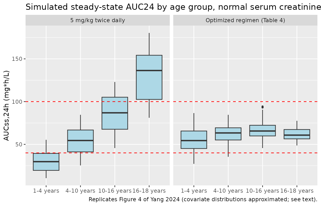
auc_fig4 |>
  dplyr::filter(regimen == "5 mg/kg twice daily") |>
  dplyr::summarise(
    sim_median = median(auc24),
    sim_p05 = quantile(auc24, 0.05),
    sim_p95 = quantile(auc24, 0.95),
    sim_pct_target = 100 * mean(auc24 >= 40 & auc24 <= 100),
    .by = age_group
  ) |>
  dplyr::left_join(fig4_groups |> dplyr::select(age_group, pub_median, pub_p05, pub_p95), by = "age_group") |>
  dplyr::rename(
    "Age group" = age_group, "Simulated median" = sim_median,
    "Simulated P5" = sim_p05, "Simulated P95" = sim_p95,
    "Simulated % in 40-100" = sim_pct_target,
    "Table S5 median" = pub_median, "Table S5 P5" = pub_p05, "Table S5 P95" = pub_p95
  ) |>
knitr::kable(digits = 1, caption = "Standard dosing (5 mg/kg twice daily): simulated vs Table S5 AUC24 (mg*h/L).")| Age group | Simulated median | Simulated P5 | Simulated P95 | Simulated % in 40-100 | Table S5 median | Table S5 P5 | Table S5 P95 |
|---|---|---|---|---|---|---|---|
| 1-4 years | 29.7 | 12.8 | 50.5 | 24.0 | 25.8 | 18.2 | 46.2 |
| 4-10 years | 54.5 | 29.2 | 77.9 | 78.0 | 44.5 | 28.1 | 69.2 |
| 10-16 years | 86.9 | 50.7 | 117.7 | 67.0 | 65.3 | 46.4 | 107.6 |
| 16-18 years | 136.4 | 87.1 | 174.0 | 20.5 | 99.7 | 78.1 | 145.3 |
The rise of exposure with age on standard mg/kg dosing, and its flattening under the optimized regimen, are reproduced. The simulated medians run about 15-40% above Table S5 because a uniform draw over each printed creatinine range places more children at the top of the range than the hospital database the paper resampled (AUC24 is almost proportional to serum creatinine). No gate is placed on this comparison for that reason; the deterministic checks above carry the validation.
Steady-state profiles and PKNCA
A cohort of 200 children per arm, with (weight, creatinine) pairs
resampled from Table S4 and between-subject variability on CL, receives
either IV GCV 5 mg/kg as a 1-h infusion or enteral VGCV 17.8 mg/kg (the
Table 1 median) every 12 h for 10 days. PKNCA computes AUC over the
final dosing interval, which at steady state equals
F x dose / CL for each child.
rxode2::rxSetSeed(20240917)
set.seed(20240917)
n_arm <- 200
make_arm <- function(arm, id_offset) {
  pick <- sample(nrow(table_s4), n_arm, replace = TRUE)
  tibble::tibble(
    id = id_offset + seq_len(n_arm),
    arm = arm,
    WT = table_s4$WT[pick],
    CREAT = table_s4$CREAT[pick]
  )
}
cohort <- dplyr::bind_rows(
  make_arm("IV GCV 5 mg/kg", 0L),
  make_arm("Enteral VGCV 17.8 mg/kg", n_arm)
)

dose_times <- seq(0, 228, by = 12)
obs_times <- sort(unique(c(seq(0, 216, by = 4), seq(228, 240, by = 0.25))))

doses <- cohort |>
  tidyr::expand_grid(time = dose_times) |>
  dplyr::mutate(
    evid = 1,
    amt = ifelse(arm == "IV GCV 5 mg/kg", 5, 17.8) * WT,
    rate = ifelse(arm == "IV GCV 5 mg/kg", amt, 0),
    cmt = ifelse(arm == "IV GCV 5 mg/kg", "central", "depot")
  )
obs <- cohort |>
  tidyr::expand_grid(time = obs_times) |>
  dplyr::mutate(evid = 0, amt = 0, rate = 0, cmt = "central")
events <- dplyr::bind_rows(doses, obs) |>
  dplyr::arrange(id, time, dplyr::desc(evid))
stopifnot(!anyDuplicated(unique(events[, c("id", "time", "evid")])))
sim <- rxode2::rxSolve(mod, events = events, keep = c("arm"), maxsteps = 1e6) |>
  as.data.frame()
#> ℹ parameter labels from comments will be replaced by 'label()'
stopifnot(!anyNA(sim$Cc))
# Steady-state interval 228-240 h; sampling windows used for TDM in the paper
# are shaded (trough 0.5-1 h pre-dose, peak 1-4 h post-dose).
sim |>
  dplyr::filter(time >= 228) |>
  dplyr::mutate(tad = time - 228) |>
  dplyr::summarise(
    Q05 = quantile(Cc, 0.05), Q50 = median(Cc), Q95 = quantile(Cc, 0.95),
    .by = c(arm, tad)
  ) |>
  ggplot(aes(tad, Q50)) +
  annotate("rect", xmin = 1, xmax = 4, ymin = 0, ymax = Inf, alpha = 0.1, fill = "darkgreen") +
  annotate("rect", xmin = 11, xmax = 11.5, ymin = 0, ymax = Inf, alpha = 0.1, fill = "darkblue") +
  geom_ribbon(aes(ymin = Q05, ymax = Q95), alpha = 0.25) +
  geom_line() +
  facet_wrap(~arm) +
  scale_y_log10() +
  labs(x = "Time after dose at steady state (h)", y = "Serum ganciclovir (mg/L)",
       title = "Steady-state profiles: median and 90% interval",
       caption = "Illustrative; the paper's Figure 2 VPC is over time since first dose of the observed TDM data.")
#> Warning in scale_y_log10(): log-10 transformation introduced infinite values.
#> log-10 transformation introduced infinite values.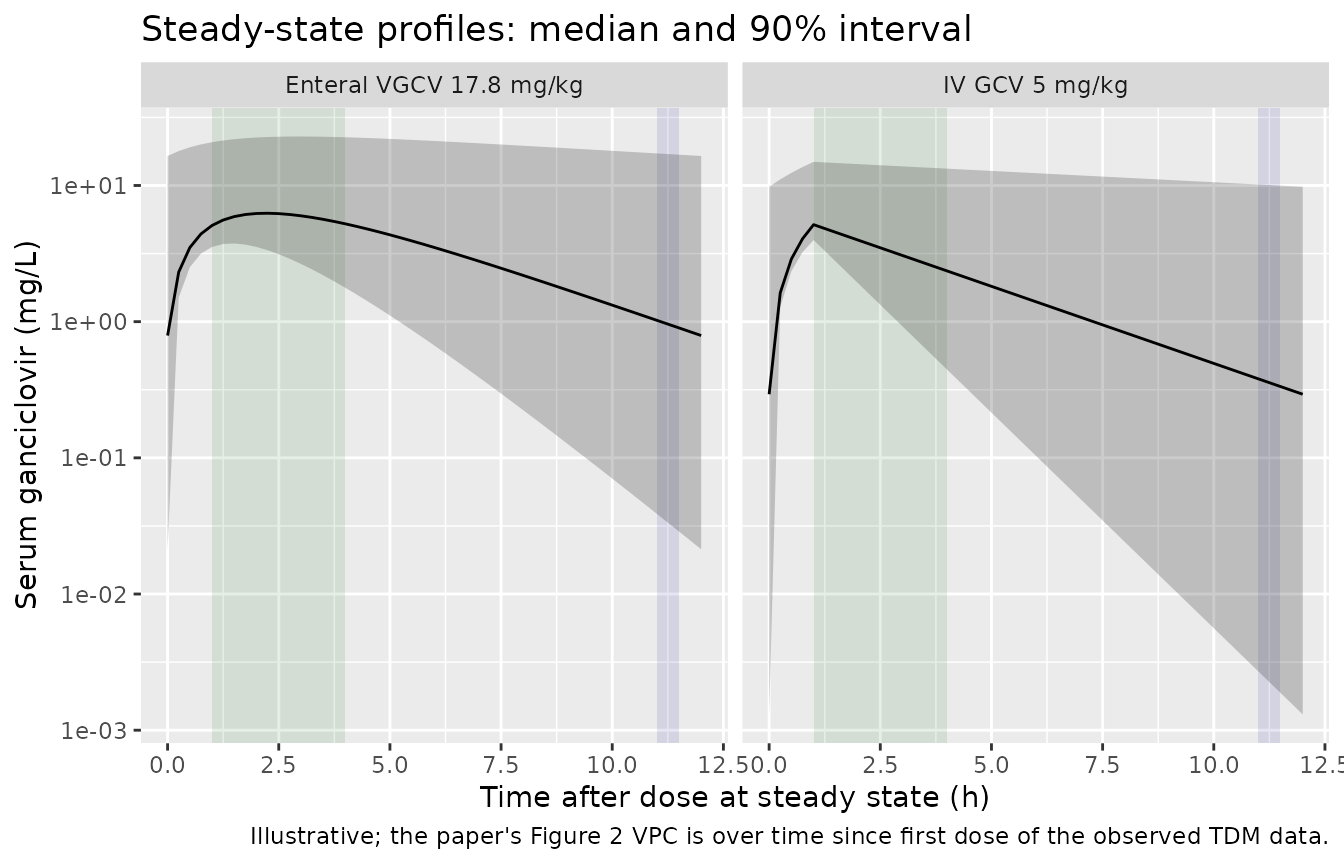
sim_nca <- sim |>
  dplyr::filter(!is.na(Cc)) |>
  dplyr::select(id, time, Cc, arm)

conc_obj <- PKNCA::PKNCAconc(sim_nca, Cc ~ time | arm + id)
dose_obj <- PKNCA::PKNCAdose(
  doses |> dplyr::select(id, time, amt, arm),
  amt ~ time | arm + id
)
intervals <- data.frame(start = 228, end = 240, auclast = TRUE, cmax = TRUE, tmax = TRUE, cmin = TRUE)
nca_res <- PKNCA::pk.nca(PKNCA::PKNCAdata(conc_obj, dose_obj, intervals = intervals))

nca_wide <- as.data.frame(nca_res) |>
  dplyr::select(id, arm, PPTESTCD, PPORRES) |>
  tidyr::pivot_wider(names_from = PPTESTCD, values_from = PPORRES)

f_vgcv <- exp(rxode2::rxode2(mod)$theta[["lfdepot"]])
#> ℹ parameter labels from comments will be replaced by 'label()'
indiv <- sim |>
  dplyr::distinct(id, cl) |>
  dplyr::left_join(
    doses |> dplyr::filter(time == 228) |> dplyr::select(id, amt, arm),
    by = "id"
  ) |>
  dplyr::mutate(auc_closed = ifelse(arm == "IV GCV 5 mg/kg", 1, f_vgcv) * amt / cl) |>
  dplyr::left_join(nca_wide |> dplyr::select(id, auclast), by = "id") |>
  dplyr::mutate(pct_diff = 100 * (auclast - auc_closed) / auc_closed)

# Same drawn parameters on both sides, so the difference is trapezoidal error
# on a 0.25-h grid plus residual accumulation after 10 days.
stopifnot(
  abs(median(indiv$pct_diff)) < 1,
  quantile(abs(indiv$pct_diff), 0.9) < 3
)

indiv |>
  dplyr::summarise(
    `Median AUC24 (mg*h/L)` = median(2 * auclast),
    `P5 AUC24` = quantile(2 * auclast, 0.05),
    `P95 AUC24` = quantile(2 * auclast, 0.95),
    `% with AUC24 40-100` = 100 * mean(2 * auclast >= 40 & 2 * auclast <= 100),
    `Median |PKNCA - closed form| (%)` = median(abs(pct_diff)),
    .by = arm
  ) |>
  dplyr::rename("Arm" = arm) |>
knitr::kable(digits = 1, caption = "Steady-state AUC24 (2 x AUC over the last 12-h interval) from PKNCA.")| Arm | Median AUC24 (mg*h/L) | P5 AUC24 | P95 AUC24 | % with AUC24 40-100 | Median |PKNCA - closed form| (%) |
|---|---|---|---|---|---|
| IV GCV 5 mg/kg | 43.0 | 15.3 | 292.4 | 25.5 | 0.0 |
| Enteral VGCV 17.8 mg/kg | 81.4 | 29.4 | 485.8 | 43.5 | 0.1 |
Comparison against published exposure
The paper reports no NCA; its exposure summary is the post hoc AUC24 on standard dosing (median 38.3 mg*h/L, 5th-95th percentile 24.8-329.2, Results).
published <- tibble::tribble(
  ~arm,             ~auclast,
  "IV GCV 5 mg/kg", 38.3 / 2
)
cmp <- nlmixr2lib::ncaComparisonTable(
  simulated = nca_res,
  reference = published,
  by = "arm",
  units = c(auclast = "mg*h/L"),
  tolerance_pct = 20
)
knitr::kable(cmp, caption = "IV arm: simulated median AUC over a 12-h interval at steady state vs half the published median post hoc AUC24. * differs from reference by >20%.")| NCA parameter | arm | Reference | Simulated | % diff |
|---|---|---|---|---|
| AUClast (mg*h/L) | IV GCV 5 mg/kg | 19.2 | 21.5 | +12.2% |
The simulated cohort resamples the same 23 children’s weight and creatinine, so its median AUC24 lands near the published post hoc median.
Assumptions and deviations
- Weight for age. The paper derived simulated children’s weights from “the observed correlation between weight and age within our patient cohort” without printing the relation. A straight line fitted by the maintainers to the Table S4 ages and weights (WT = 1.139 + 3.823 x age, kg and years) is used. With mg/kg dosing, AUC24 depends on weight only as WT^0.25, so this choice barely affects any result above.
- Serum creatinine distributions for Figure 4 / Table S5 come from an unpublished hospital database; uniform draws over the printed normal ranges are used, which biases the simulated medians upward (see the Figure 4 section).
- Table S4 gives the 22nd child the number 21 (a duplicate); it is renumbered 22. Its serum creatinine is presumably the baseline value, whereas the post hoc AUC used the time-varying value.
-
Valganciclovir dose units. Enteral doses are
milligrams of valganciclovir into
depot; the fixed F = 0.536 includes the molecular-weight ratio, as in the source. - Renal replacement therapy was tested on CL and not retained (OFV change 0.056; Discussion), so the model has no RRT term.
- Figure 2 (VPC over time since first dose of the TDM data) cannot be rebuilt without the individual dosing histories; the steady-state profile plot is illustrative only.
- No correction notice for the article was found in Europe PMC as of 2026-10-30.