MEN1611 + trastuzumab xenograft tumor growth inhibition (Tosca 2023)
Source:vignettes/articles/Tosca_2023_men1611_trastuzumab.Rmd
Tosca_2023_men1611_trastuzumab.RmdModel and source
- Citation: Tosca EM, Borella E, Piana C, Bouchene S, Merlino G, Fiascarelli A, Mazzei P, Magni P. Model-based prediction of effective target exposure for MEN1611 in combination with trastuzumab in HER2-positive advanced or metastatic breast cancer patients. CPT Pharmacometrics Syst Pharmacol. 2023;12(11):1626-1639. doi:10.1002/psp4.12910. Tumor parameters from Table 2; PK parameters from Supplementary Tables S3 (trastuzumab) and S4 (MEN1611); equations from Equations 2-3 and Supplementary Material S3. Growth model from Simeoni M, et al. Cancer Res. 2004;64(3):1094-1101. doi:10.1158/0008-5472.CAN-03-2524.
- Article: CPT Pharmacometrics Syst Pharmacol. 2023;12(11):1626-1639 (open access; PMC10681519)
Tosca et al. built a translational PK-PD framework to find the MEN1611 exposure that, given together with trastuzumab, eradicates HER2-positive, trastuzumab-resistant, PI3K-pathway-mutated breast-cancer xenografts, and then carried that exposure to patients. The paper contributes nine model files:
| Model file | What it is | Source |
|---|---|---|
Tosca_2023_men1611_mouse |
MEN1611 two-compartment PK in tumor-free mice (IV, oral solution, oral suspension) | Table S4 |
Tosca_2023_trastuzumab_mouse |
Trastuzumab two-compartment PK in tumor-bearing mice (IV, intraperitoneal) | Table S3 |
Tosca_2023_men1611_trastuzumab_kpl4_mouse |
2D tumor growth inhibition, TGI study A (KPL-4), synergistic | Table 2 |
Tosca_2023_men1611_trastuzumab_jimt1_mouse |
TGI study B (JIMT-1), synergistic | Table 2 |
Tosca_2023_men1611_trastuzumab_hcc1954_mouse |
TGI study C (HCC1954), synergistic | Table 2 |
Tosca_2023_men1611_trastuzumab_ctg0033_mouse |
TGI study D (CTG-0033 PDX), synergistic | Table 2 |
Tosca_2023_men1611_trastuzumab_bcpdx67_mouse |
TGI study E (BC-PDX-67), synergistic | Table 2 |
Tosca_2023_men1611_trastuzumab_pdx153_mouse |
TGI study F (PDX-153), additive | Table 2 |
Tosca_2023_men1611_trastuzumab_pdx173jal_mouse |
TGI study G (PDX-173-JAL), additive | Table 2 |
The seven xenograft studies were analysed separately, each with its own growth and drug-effect parameters, so each is its own model file. Every TGI file carries both mouse PK models with their parameters held fixed, because the authors used the typical PK profiles as the input to the tumor model.
Population
All data are preclinical (mouse). MEN1611 PK came from two studies in tumor-free mice: study 1 gave a DMSO solution IV (2 mg/kg, 2 animals) or orally (0.5, 1, 2 or 5 mg/kg, 4 animals per group) to BALB-nu/nu mice; study 2 gave an MCT suspension orally once daily for 5 days (1.25, 6.25 or 12.5 mg/kg, 12 CD-1 mice per group). Trastuzumab PK came from two literature studies in tumor-bearing mice (single IV doses of 3.43 to 383.68 ug with 111In- and 125I-trastuzumab; a single IP dose of 17.65 ug of 86Y-trastuzumab), converted from radioactivity per gram of blood to plasma ng/mL (Material S1).
The seven TGI studies (Table 1) used three cell-line-derived and four patient-derived xenografts of HER2-amplified, trastuzumab-resistant breast cancer, each with a vehicle, MEN1611, trastuzumab and combination arm (4 to 10 mice per arm, 188 mice in total). MEN1611 was given orally at 6.5 mg/kg (12.5 mg/kg in study A) once daily for 12 days (6 weeks in study G); trastuzumab was given at 30 mg/kg weekly (IV in study A, IP in B-D) or 10 mg/kg IP (studies E-G).
Source trace
| Element | Source location | Value |
|---|---|---|
| MEN1611 PK: Kabs, CL, V1, Q, V2 | Table S4 | 1.84 1/h, 1 L/h/kg, 0.997 L/kg, 1.49 L/h/kg, 7.6 L/kg |
| MEN1611 F (solution / suspension) | Table S4 | 1 (fixed) / 0.559 |
| MEN1611 residual error a, b | Table S4; combined form from Methods | 1.66 ng/mL, 0.476 |
| Trastuzumab PK: F, Kabs, V1, CL, Q, V2 | Table S3 | 0.5557, 0.151 1/h, 2.45e-3 L, 1.53e-5 L/h, 2.58e-4 L/h, 2.22e-3 L |
| Trastuzumab residual error b | Table S3 | 0.095 (proportional) |
| Simeoni growth and single-drug chain | Material S3 ‘Perturbed growth model’ | – |
| Additive 2D mortality grid | Material S3 ‘Additive 2D-TGI model’ | – |
| Synergistic potency k2,TZB,combo = k2,TZB (1 + gamma C_MEN1611) | Equations 2-3 | – |
| lambda0, lambda1, W0, k1, k2, gamma per study | Table 2 | see each model file |
| k2,TZB for study G | Results text range and Table 3 (Table 2 prints ‘8888’) | 7.08e-7 mL/(ng day) |
| psi | Simeoni 2004 (not printed in Tosca 2023) | 20 |
| Effective concentration C_MEN1611,eff | Equations 4 (additive) and 5 (synergistic) | – |
| Effective exposure AUC0-12h = 12 h x C_MEN1611,eff | Equation 6 | – |
| Clinical trastuzumab steady-state concentrations | Table S2 | – |
MEN1611 PK in mice
mod_men <- rxode2::rxode2(readModelDb("Tosca_2023_men1611_mouse"))

# Study 1 (DMSO solution, single dose) and study 2 (MCT suspension, day 1).
men_groups <- tibble::tribble(
  ~id, ~arm,                     ~amt, ~cmt,      ~FORM_SOLUTION,
  1,   "2 mg/kg IV",               2,  "central", 1,
  2,   "0.5 mg/kg PO solution",  0.5,  "depot",   1,
  3,   "1 mg/kg PO solution",      1,  "depot",   1,
  4,   "2 mg/kg PO solution",      2,  "depot",   1,
  5,   "5 mg/kg PO solution",      5,  "depot",   1,
  6,   "1.25 mg/kg PO suspension", 1.25, "depot", 0,
  7,   "6.25 mg/kg PO suspension", 6.25, "depot", 0,
  8,   "12.5 mg/kg PO suspension", 12.5, "depot", 0
)
obs_times <- sort(unique(c(seq(0, 2, by = 0.02), seq(2, 48, by = 0.25))))
men_ev <- bind_rows(
  men_groups |> mutate(time = 0, evid = 1),
  tidyr::expand_grid(men_groups |> select(id, arm, FORM_SOLUTION), time = obs_times) |>
    mutate(evid = 0, amt = 0, cmt = "central")
) |>
  arrange(id, time, desc(evid))
men_sim <- rxSolve(mod_men, men_ev, keep = "arm", returnType = "data.frame")
#> Warning: multi-subject simulation without without 'omega'
ggplot(filter(men_sim, time <= 24, Cc >= 1e-3), aes(time, Cc, colour = arm)) +
  geom_line() +
  scale_y_log10() +
  labs(x = "Time (h)", y = "MEN1611 plasma concentration (ng/mL)", colour = NULL) +
  theme_bw()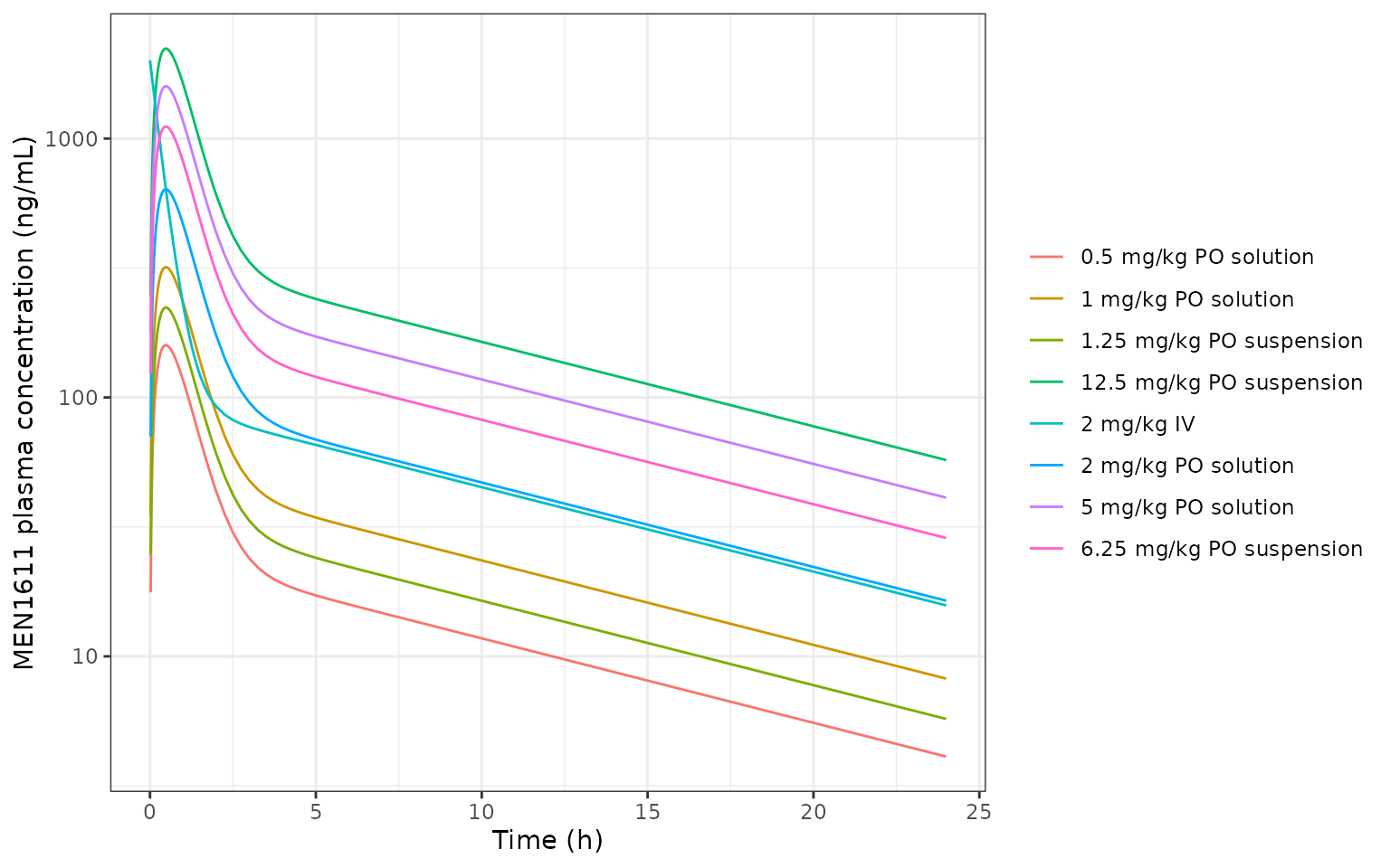
Typical MEN1611 plasma concentrations in mice. Replicates the model lines of Figures S11 (solution, study 1) and S12 day 1 (suspension, study 2) of Tosca 2023.
Trastuzumab PK in mice
mod_tzb <- rxode2::rxode2(readModelDb("Tosca_2023_trastuzumab_mouse"))

# Total (labelled + unlabelled) doses in ug from Material S1, given here in mg.
tzb_groups <- tibble::tribble(
  ~id, ~arm,               ~amt,      ~cmt,
  1,   "3.43 ug IV",      0.00343,   "central",
  2,   "32.68 ug IV",     0.03268,   "central",
  3,   "383.68 ug IV",    0.38368,   "central",
  4,   "17.65 ug IP",     0.01765,   "depot"
)
tzb_times <- sort(unique(c(seq(0, 24, by = 0.1), seq(24, 3000, by = 2))))
tzb_ev <- bind_rows(
  tzb_groups |> mutate(time = 0, evid = 1),
  tidyr::expand_grid(tzb_groups |> select(id, arm), time = tzb_times) |>
    mutate(evid = 0, amt = 0, cmt = "central")
) |>
  arrange(id, time, desc(evid))
tzb_sim <- rxSolve(mod_tzb, tzb_ev, keep = "arm", returnType = "data.frame")
#> Warning: multi-subject simulation without without 'omega'
ggplot(filter(tzb_sim, time <= 200, Cc >= 1e-3), aes(time, Cc, colour = arm)) +
  geom_line() +
  scale_y_log10() +
  labs(x = "Time (h)", y = "Trastuzumab plasma concentration (ng/mL)", colour = NULL) +
  theme_bw()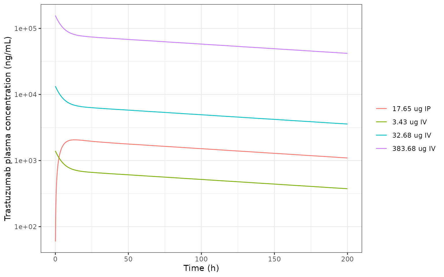
Typical trastuzumab plasma concentrations in mice. Replicates the model lines of Figure S8 of Tosca 2023.
Comparison with the supplementary PK figures
The paper prints no NCA table. The model lines of Figures S8, S9, S11 and S12 were read off the plotted curves by the maintainers; readings are approximate (roughly 5-10% at these axis scales).
pk_checks <- bind_rows(
  tibble(
    check = "Trastuzumab 383.68 ug IV, concentration at 0.1 h (Fig S9A)",
    published = 150000,
    simulated = filter(tzb_sim, arm == "383.68 ug IV", abs(time - 0.1) < 1e-6)$Cc
  ),
  tibble(
    check = "Trastuzumab 17.65 ug IP, peak (Fig S9B)",
    published = 2050,
    simulated = max(filter(tzb_sim, arm == "17.65 ug IP")$Cc)
  ),
  tibble(
    check = "Trastuzumab 17.65 ug IP, concentration at 200 h (Fig S9B)",
    published = 1100,
    simulated = filter(tzb_sim, arm == "17.65 ug IP", time == 200)$Cc
  ),
  tibble(
    check = "MEN1611 5 mg/kg PO solution, peak (Fig S11A)",
    published = 1500,
    simulated = max(filter(men_sim, arm == "5 mg/kg PO solution")$Cc)
  ),
  tibble(
    check = "MEN1611 2 mg/kg IV, concentration at 24 h (Fig S11B)",
    published = 16,
    simulated = filter(men_sim, arm == "2 mg/kg IV", time == 24)$Cc
  ),
  tibble(
    check = "MEN1611 12.5 mg/kg PO suspension, day-1 peak (Fig S12A)",
    published = 2350,
    simulated = max(filter(men_sim, arm == "12.5 mg/kg PO suspension")$Cc)
  )
) |>
  mutate(pct_diff = 100 * (simulated - published) / published)

pk_checks |>
  mutate(simulated = signif(simulated, 4), pct_diff = round(pct_diff, 1)) |>
  rename(
    "Check" = check, "Read from figure (ng/mL)" = published,
    "Simulated (ng/mL)" = simulated, "Difference (%)" = pct_diff
  ) |>
knitr::kable()| Check | Read from figure (ng/mL) | Simulated (ng/mL) | Difference (%) |
|---|---|---|---|
| Trastuzumab 383.68 ug IV, concentration at 0.1 h (Fig S9A) | 150000 | 154900.00 | 3.3 |
| Trastuzumab 17.65 ug IP, peak (Fig S9B) | 2050 | 2057.00 | 0.4 |
| Trastuzumab 17.65 ug IP, concentration at 200 h (Fig S9B) | 1100 | 1094.00 | -0.5 |
| MEN1611 5 mg/kg PO solution, peak (Fig S11A) | 1500 | 1592.00 | 6.2 |
| MEN1611 2 mg/kg IV, concentration at 24 h (Fig S11B) | 16 | 15.73 | -1.7 |
| MEN1611 12.5 mg/kg PO suspension, day-1 peak (Fig S12A) | 2350 | 2225.00 | -5.3 |
PKNCA
PKNCA confirms the dose-linearity of the PK models and the two bioavailabilities: for the MEN1611 IV dose, AUC0-inf must equal dose / CL (2 mg/kg / 1 L/h/kg = 2000 ng h/mL), and the suspension’s dose-normalised AUC must be 0.559 times the solution’s.
men_conc <- men_sim |>
  select(id, time, Cc, arm) |>
  filter(!is.na(Cc))
men_dose <- men_groups |>
  mutate(time = 0) |>
  select(id, time, amt, arm)

conc_obj <- PKNCAconc(men_conc, Cc ~ time | arm + id)
dose_obj <- PKNCAdose(men_dose, amt ~ time | arm + id)
intervals <- data.frame(
  start = 0, end = Inf,
  cmax = TRUE, tmax = TRUE, aucinf.obs = TRUE, half.life = TRUE
)
men_nca <- pk.nca(PKNCAdata(conc_obj, dose_obj, intervals = intervals))
men_nca_wide <- as.data.frame(men_nca$result) |>
  select(arm, PPTESTCD, PPORRES) |>
  pivot_wider(names_from = PPTESTCD, values_from = PPORRES) |>
  left_join(select(men_groups, arm, amt), by = "arm") |>
  mutate(auc_per_dose = aucinf.obs / amt)

men_nca_wide |>
  mutate(across(c(cmax, aucinf.obs, half.life, auc_per_dose), ~ signif(.x, 4))) |>
  select(arm, cmax, tmax, aucinf.obs, half.life, auc_per_dose) |>
  rename(
    "Group" = arm, "Cmax (ng/mL)" = cmax, "Tmax (h)" = tmax,
    "AUC0-inf (ng h/mL)" = aucinf.obs, "t1/2 (h)" = half.life,
    "AUC0-inf / dose" = auc_per_dose
  ) |>
knitr::kable()| Group | Cmax (ng/mL) | Tmax (h) | AUC0-inf (ng h/mL) | t1/2 (h) | AUC0-inf / dose |
|---|---|---|---|---|---|
| 0.5 mg/kg PO solution | 159.2 | 0.48 | 500.1 | 9.208 | 1000.0 |
| 1 mg/kg PO solution | 318.5 | 0.48 | 1000.0 | 9.208 | 1000.0 |
| 1.25 mg/kg PO suspension | 222.5 | 0.48 | 698.8 | 9.208 | 559.1 |
| 12.5 mg/kg PO suspension | 2225.0 | 0.48 | 6988.0 | 9.208 | 559.1 |
| 2 mg/kg IV | 2006.0 | 0.00 | 2000.0 | 9.208 | 1000.0 |
| 2 mg/kg PO solution | 637.0 | 0.48 | 2000.0 | 9.208 | 1000.0 |
| 5 mg/kg PO solution | 1592.0 | 0.48 | 5001.0 | 9.208 | 1000.0 |
| 6.25 mg/kg PO suspension | 1113.0 | 0.48 | 3494.0 | 9.208 | 559.1 |
auc_iv <- men_nca_wide$aucinf.obs[men_nca_wide$arm == "2 mg/kg IV"]
apd_sol <- men_nca_wide$auc_per_dose[grepl("solution", men_nca_wide$arm)]
apd_susp <- men_nca_wide$auc_per_dose[grepl("suspension", men_nca_wide$arm)]
stopifnot(
  abs(auc_iv / 2000 - 1) < 0.01,
  abs(mean(apd_sol) / (auc_iv / 2) - 1) < 0.01,
  abs(mean(apd_susp) / mean(apd_sol) - 0.559) < 0.005
)
Tumor growth inhibition in the seven xenografts
Structure
Each TGI file follows Material S3. Without treatment the tumor weight
W grows exponentially at rate lambda0 and then linearly at
rate lambda1 (Simeoni 2004, with psi = 20); studies B-E never reached
the linear phase and use exponential growth only. MEN1611 and
trastuzumab each move proliferating cells (cycling_cells)
into a three-stage mortality chain at a rate k2 * C(t), and
damaged cells progress along that chain at k1. Because a
cell hit by one drug can still be hit by the other, the damaged cells
form a four-by-four grid:
damaged_cells_m<i>_t<j> has progressed
i stages along the MEN1611 chain and j along
the trastuzumab chain (paper compartment X_(i+1)(j+1)). The
observed tumor weight is the sum of all 16 states.
In studies A-E the combination arm grew more slowly than this
additive grid predicts, so the authors added a synergy term (Equation
3): the trastuzumab potency becomes
k2,TZB (1 + gamma C_MEN1611), i.e. MEN1611 restores
trastuzumab activity in proportion to its concentration. Studies F and G
showed no synergy and keep the additive grid.
Dosing used in the simulations
Treatment start days and the shape of each schedule were read from the dosing triangles of Figure 1; doses and regimens are from Table 1. Table 1’s ‘q2w’ is plotted as two doses a week, and is simulated that way. Trastuzumab doses in mg/kg are converted to mg per mouse with the 22.5 g body weight the paper uses for the PK data.
tgi_design <- tibble::tribble(
  ~study, ~stem,       ~line,         ~start, ~men_dose, ~men_days, ~tzb_dose, ~tzb_route, ~tzb_times,        ~tend, ~w0_tzb, ~w0_men,
  "A",    "kpl4",      "KPL-4",           20, 12.5,      12,        30,        "IV",       "0,7",               90,  NA,      NA,
  "B",    "jimt1",     "JIMT-1",          15, 6.5,       12,        30,        "IP",       "0,7",               50,  NA,      NA,
  "C",    "hcc1954",   "HCC1954",         15, 6.5,       12,        30,        "IP",       "0,7",               50,  NA,      NA,
  "D",    "ctg0033",   "CTG-0033",        15, 6.5,       12,        30,        "IP",       "0,7",               50,  NA,      NA,
  "E",    "bcpdx67",   "BC-PDX-67",       33, 6.5,       12,        10,        "IP",       "0,3.5,7,10.5",      80,  NA,      NA,
  "F",    "pdx153",    "PDX-153",         61, 6.5,       12,        10,        "IP",       "0,3.5,7,10.5,14,17.5", 137, 0.025, 0.024,
  "G",    "pdx173jal", "PDX-173-JAL",     34, 6.5,       42,        10,        "IP",       "0,3.5,7,10.5,14,17.5", 76,  0.01,  0.004
)
mouse_wt_kg <- 0.0225
arms <- c("Control", "MEN1611", "Trastuzumab", "MEN1611 + trastuzumab")

tgi_events <- function(d, arm, grid = seq(0, d$tend, by = 0.25)) {
  obs <- et(grid)
  if (arm %in% c("MEN1611", "MEN1611 + trastuzumab")) {
    obs <- obs |>
      et(amt = d$men_dose, cmt = "depot_men1611", time = d$start, ii = 1, addl = d$men_days - 1)
  }
  if (arm %in% c("Trastuzumab", "MEN1611 + trastuzumab")) {
    tzb_cmt <- if (d$tzb_route == "IV") "central_trastuzumab" else "depot_trastuzumab"
    for (tt in as.numeric(strsplit(d$tzb_times, ",")[[1]])) {
      obs <- obs |> et(amt = d$tzb_dose * mouse_wt_kg, cmt = tzb_cmt, time = d$start + tt)
    }
  }
  obs
}

# Table 2 reports a separate W0 for each single-agent arm of studies F and G;
# the control-arm W0 carried in the model is used for the control and
# combination arms.
tgi_params <- function(d, arm) {
  w0 <- switch(arm,
    "Trastuzumab" = d$w0_tzb,
    "MEN1611" = d$w0_men,
    NA
  )
  if (is.na(w0)) NULL else c(lrbase_tumor = log(w0))
}

tgi_solve <- function(d, arm, mod, extra = NULL) {
  p <- c(tgi_params(d, arm), extra)
  out <- if (is.null(p)) {
    rxSolve(mod, tgi_events(d, arm), returnType = "data.frame")
  } else {
    rxSolve(mod, tgi_events(d, arm), params = p, returnType = "data.frame")
  }
  out |>
    mutate(study = d$study, line = d$line, arm = arm) |>
    select(study, line, arm, time, tumor_size, Cc_men1611, Cc_trastuzumab)
}

tgi_models <- lapply(tgi_design$stem, function(s) {
  rxode2::rxode2(readModelDb(paste0("Tosca_2023_men1611_trastuzumab_", s, "_mouse")))
})
names(tgi_models) <- tgi_design$study

tgi_sim <- bind_rows(lapply(seq_len(nrow(tgi_design)), function(i) {
  d <- tgi_design[i, ]
  bind_rows(lapply(arms, function(a) tgi_solve(d, a, tgi_models[[d$study]])))
})) |>
  mutate(arm = factor(arm, levels = arms), panel = paste0("Study ", study, ": ", line))
ggplot(tgi_sim, aes(time, tumor_size, colour = arm)) +
  geom_line() +
  facet_wrap(~panel, scales = "free") +
  labs(x = "Time (days)", y = "Tumor weight (g)", colour = NULL) +
  theme_bw() +
  theme(legend.position = "bottom")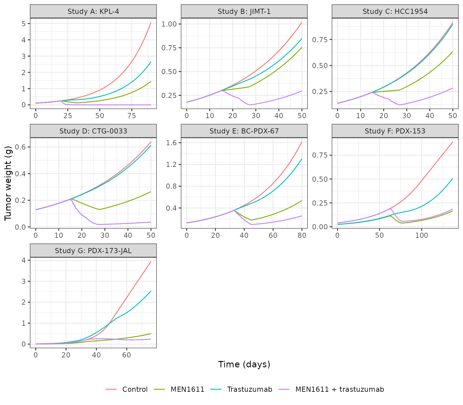
Typical tumor weight by arm in each xenograft study. Replicates the model lines of Figure 4a and Figures S14 and S19 of Tosca 2023 (combination arms of studies A-E with the synergistic model; studies F-G with the additive model).
Additive versus synergistic prediction for the combination arms
Figure 4b and Figure S18 overlay the additive (no-interaction) prediction on the combination-arm data, and Figure 4c and Figure S19 the synergistic fit. Setting the synergy factor to zero in a study A-E file gives the additive prediction.
syn_studies <- tgi_design |> filter(study %in% c("A", "B", "C", "D", "E"))
combo_cmp <- bind_rows(lapply(seq_len(nrow(syn_studies)), function(i) {
  d <- syn_studies[i, ]
  m <- tgi_models[[d$study]]
  bind_rows(
    tgi_solve(d, "MEN1611 + trastuzumab", m) |> mutate(model = "Synergistic"),
    tgi_solve(d, "MEN1611 + trastuzumab", m, extra = c(lsynergy = log(1e-30))) |>
      mutate(model = "Additive (gamma = 0)")
  )
})) |>
  mutate(panel = paste0("Study ", study, ": ", line))

ggplot(combo_cmp, aes(time, tumor_size, colour = model)) +
  geom_line() +
  facet_wrap(~panel, scales = "free") +
  labs(x = "Time (days)", y = "Tumor weight (g)", colour = NULL) +
  theme_bw() +
  theme(legend.position = "bottom")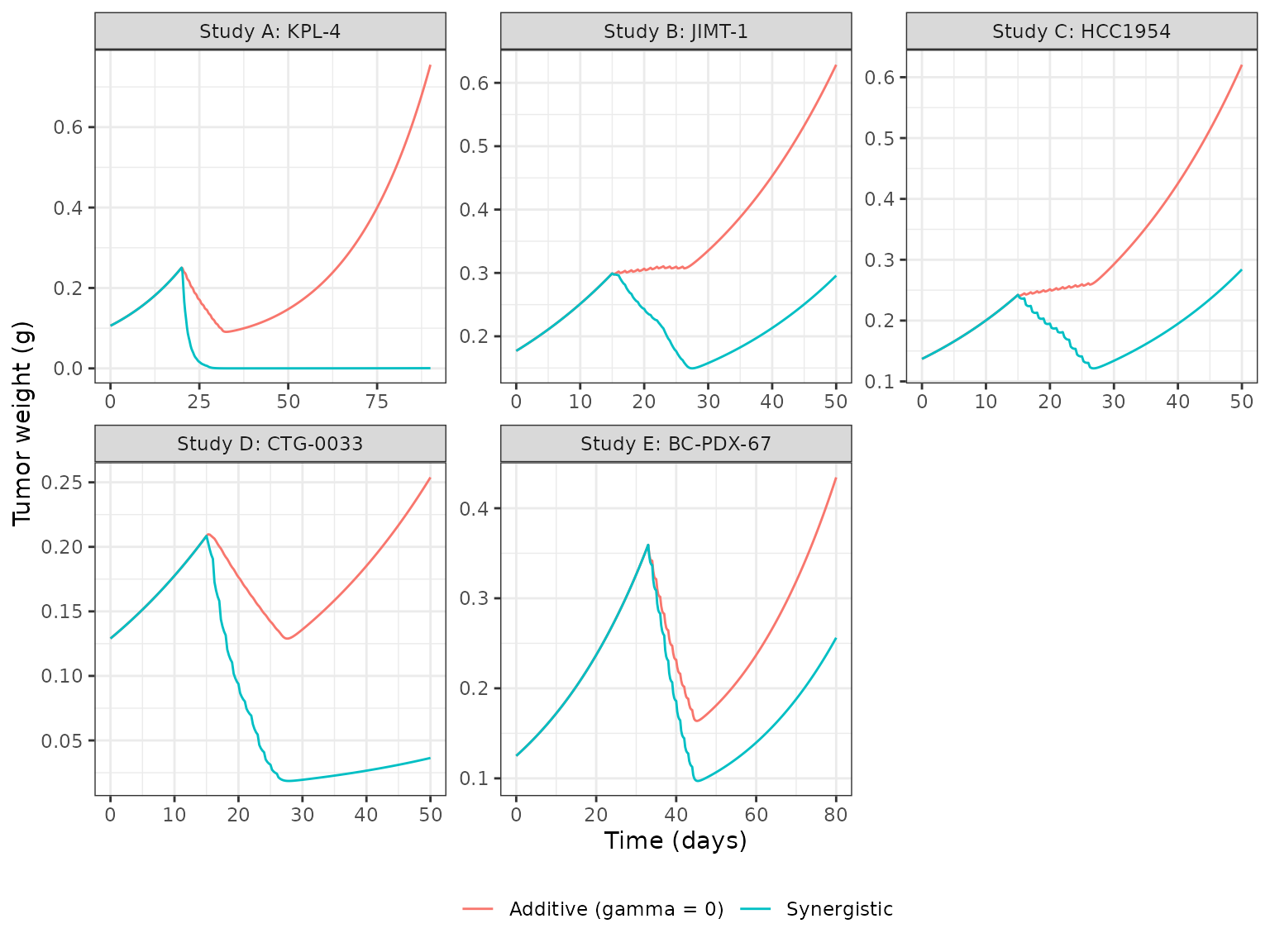
Combination arms of studies A-E: additive prediction (gamma = 0; Figure 4b and S18 of Tosca 2023) against the synergistic model (Figure 4c and S19).
combo_end <- combo_cmp |>
  group_by(study, model) |>
  filter(time == max(time)) |>
  ungroup() |>
  select(study, model, tumor_size) |>
  pivot_wider(names_from = model, values_from = tumor_size)
# The synergy term is what the paper added to explain combination arms that
# grew far less than the additive prediction; it must shrink the tumor.
stopifnot(all(combo_end$Synergistic < 0.8 * combo_end$`Additive (gamma = 0)`))
Comparison with the supplementary TGI figures
The model lines of Figure 4a (study A control) and Figure S14 (studies B-G) were read off the plotted curves by the maintainers at the end of each curve. Control arms depend only on lambda0, lambda1, psi and W0; the MEN1611 arms also test the PK chain, the MEN1611 potency and the dosing schedule reconstructed above. Figure S14’s legend in panels B-F swaps the MEN1611 and trastuzumab colours relative to its caption and panel G; the caption’s assignment (MEN1611 green) is the one consistent with the parameter estimates and is used here.
tgi_read <- tibble::tribble(
  ~study, ~arm,          ~time, ~published,
  "A",    "Control",        90, 4.9,
  "B",    "Control",        50, 1.00,
  "C",    "Control",        50, 0.92,
  "D",    "Control",        50, 0.65,
  "E",    "Control",        80, 1.63,
  "F",    "Control",       137, 0.95,
  "G",    "Control",        55, 1.78,
  "B",    "MEN1611",        50, 0.75,
  "C",    "MEN1611",        50, 0.63,
  "D",    "MEN1611",        50, 0.27,
  "E",    "MEN1611",        80, 0.55,
  "F",    "MEN1611",       137, 0.18,
  "G",    "MEN1611",        70, 0.63
)
tgi_cmp <- tgi_read |>
  left_join(
    tgi_sim |> mutate(arm = as.character(arm)) |> select(study, arm, time, tumor_size),
    by = c("study", "arm", "time")
  ) |>
  mutate(pct_diff = 100 * (tumor_size - published) / published)

tgi_cmp |>
  mutate(tumor_size = signif(tumor_size, 3), pct_diff = round(pct_diff, 1)) |>
  rename(
    "Study" = study, "Arm" = arm, "Day" = time,
    "Read from figure (g)" = published, "Simulated (g)" = tumor_size,
    "Difference (%)" = pct_diff
  ) |>
knitr::kable()| Study | Arm | Day | Read from figure (g) | Simulated (g) | Difference (%) |
|---|---|---|---|---|---|
| A | Control | 90 | 4.90 | 5.080 | 3.7 |
| B | Control | 50 | 1.00 | 1.020 | 1.9 |
| C | Control | 50 | 0.92 | 0.916 | -0.4 |
| D | Control | 50 | 0.65 | 0.639 | -1.7 |
| E | Control | 80 | 1.63 | 1.620 | -0.8 |
| F | Control | 137 | 0.95 | 0.890 | -6.3 |
| G | Control | 55 | 1.78 | 1.680 | -5.6 |
| B | MEN1611 | 50 | 0.75 | 0.755 | 0.7 |
| C | MEN1611 | 50 | 0.63 | 0.634 | 0.7 |
| D | MEN1611 | 50 | 0.27 | 0.265 | -1.9 |
| E | MEN1611 | 80 | 0.55 | 0.537 | -2.3 |
| F | MEN1611 | 137 | 0.18 | 0.168 | -6.9 |
| G | MEN1611 | 70 | 0.63 | 0.416 | -34.0 |
ctrl <- filter(tgi_cmp, arm == "Control")
men <- filter(tgi_cmp, arm == "MEN1611")
stopifnot(
  # Control growth: lambda0 and W0 enter exponentially, so a transcription
  # error in either moves the late weight by far more than the reading error.
  abs(median(ctrl$pct_diff)) < 10,
  max(abs(ctrl$pct_diff)) < 20,
  # Treated arms also carry the reconstructed dosing schedule.
  abs(median(men$pct_diff)) < 20
)
The one treated arm that misses is study G’s MEN1611 arm, and it is the one whose schedule is least certain. Table 1 says once daily for 6 weeks, while the dosing triangles of Figure S14 show weekday dosing (days 34-35, then five-day blocks through day 69). The two schedules bracket the published curve:
d_g <- filter(tgi_design, study == "G")
g_schedules <- list(
  "Daily for 6 weeks (Table 1)" = d_g$start + 0:41,
  "Weekdays, days 34-69 (Figure S14)" = c(34, 35, 37:41, 44:48, 51:55, 58:62, 65:69)
)
g_read <- tibble(time = c(50, 60, 70), published = c(0.28, 0.40, 0.64))
g_cmp <- bind_rows(lapply(names(g_schedules), function(nm) {
  ev <- et(g_read$time)
  for (t in g_schedules[[nm]]) {
    ev <- et(ev, amt = d_g$men_dose, cmt = "depot_men1611", time = t)
  }
  out <- rxSolve(tgi_models[["G"]], ev,
    params = c(lrbase_tumor = log(d_g$w0_men)), returnType = "data.frame"
  )
  tibble(schedule = nm, time = out$time, simulated = out$tumor_size)
})) |>
  left_join(g_read, by = "time")

g_cmp |>
  mutate(simulated = signif(simulated, 3)) |>
  pivot_wider(names_from = schedule, values_from = simulated) |>
  rename("Day" = time, "Read from Figure S14 (g)" = published) |>
knitr::kable()| Day | Read from Figure S14 (g) | Daily for 6 weeks (Table 1) | Weekdays, days 34-69 (Figure S14) |
|---|---|---|---|
| 50 | 0.28 | 0.218 | 0.285 |
| 60 | 0.40 | 0.301 | 0.489 |
| 70 | 0.64 | 0.416 | 0.778 |
Maximum restored trastuzumab potency (Table S9)
Table S9 lists the largest value of k2,TZB,combo reached
in each synergistic combination arm, which by Equation 3 occurs at the
MEN1611 peak. This is a direct test of the MEN1611 PK in the TGI files
and of the unit of gamma: it reproduces the table only with the MEN1611
clearances read per kg, the solution bioavailability of 1, and gamma in
mL/ng.
s9_pub <- c(A = 3.24e-5, B = 6.59e-6, C = 7.19e-6, D = 1.67e-5, E = 8.5e-6)
# The MEN1611 peak comes about an hour after each dose, so it needs a grid
# much finer than the 0.25-day plotting grid.
s9_peak <- bind_rows(lapply(names(s9_pub), function(s) {
  d <- filter(tgi_design, study == s)
  fine <- seq(d$start, d$start + d$men_days, by = 0.002)
  out <- rxSolve(
    tgi_models[[s]], tgi_events(d, "MEN1611 + trastuzumab", grid = fine),
    returnType = "data.frame"
  )
  tibble(study = s, cmax_men1611 = max(out$Cc_men1611))
}))
s9 <- s9_peak |>
  rowwise() |>
  mutate(
    k2_tzb = exp(tgi_models[[study]]$theta[["ldrugSlope_trastuzumab"]]),
    gamma = exp(tgi_models[[study]]$theta[["lsynergy"]]),
    simulated = k2_tzb * (1 + gamma * cmax_men1611),
    published = s9_pub[[study]],
    pct_diff = 100 * (simulated - published) / published
  ) |>
  ungroup()

s9 |>
  mutate(across(c(cmax_men1611, simulated), ~ signif(.x, 4)), pct_diff = round(pct_diff, 1)) |>
  select(study, cmax_men1611, published, simulated, pct_diff) |>
  rename(
    "Study" = study, "Peak MEN1611 (ng/mL)" = cmax_men1611,
    "Table S9 max k2,TZB,combo" = published, "Simulated" = simulated,
    "Difference (%)" = pct_diff
  ) |>
knitr::kable()| Study | Peak MEN1611 (ng/mL) | Table S9 max k2,TZB,combo | Simulated | Difference (%) |
|---|---|---|---|---|
| A | 4100 | 3.24e-05 | 3.12e-05 | -3.7 |
| B | 2132 | 6.60e-06 | 6.60e-06 | 0.0 |
| C | 2132 | 7.20e-06 | 6.70e-06 | -6.3 |
| D | 2132 | 1.67e-05 | 1.67e-05 | 0.3 |
| E | 2132 | 8.50e-06 | 8.50e-06 | 0.0 |
Studies B, D and E match to the printed precision. Study C’s 6% gap follows from the one-significant-figure k2,TZB printed in Table 2 (1.2E-8), and study A’s 4% gap is consistent with the study A discrepancy in the effective-exposure tables below.
Effective MEN1611 exposures in patients (Table 3, S6, S7)
Holding both concentrations constant, the tumor is eradicated when
the kill rate exceeds lambda0, which gives the minimal effective MEN1611
concentration C_eff = (lambda0 - k2,TZB C_TZB) / k2,MEN1611
for the additive model (Equation 4) and
C_eff = (lambda0 - k2,TZB C_TZB) / (k2,MEN1611 + gamma k2,TZB C_TZB)
for the synergistic model (Equation 5); a negative value means
trastuzumab alone suffices, and is reported as 0. The effective
twice-daily exposure is AUC0-12h = 12 h x C_eff (Equation
6). Trastuzumab concentrations are the clinical steady-state values of
Table S2.
ctzb <- tibble::tribble(
  ~regimen,                              ~scenario,                ~bound,  ~ctzb_ugml,
  "IV 4 mg/kg + 2 mg/kg q1w (Table 3)",  "1: C_TZB,ss,avg",        "point", 81.43,
  "IV 4 mg/kg + 2 mg/kg q1w (Table 3)",  "2: C_TZB,min / C_TZB,max", "low",  107,
  "IV 4 mg/kg + 2 mg/kg q1w (Table 3)",  "2: C_TZB,min / C_TZB,max", "high", 63.1,
  "IV 4 mg/kg + 2 mg/kg q1w (Table 3)",  "3: 90% CI of C_TZB,ss,avg", "low",  129.3,
  "IV 4 mg/kg + 2 mg/kg q1w (Table 3)",  "3: 90% CI of C_TZB,ss,avg", "high", 27.7,
  "IV 8 mg/kg + 6 mg/kg q3w (Table S6)", "1: C_TZB,ss,avg",        "point", 82.66,
  "IV 8 mg/kg + 6 mg/kg q3w (Table S6)", "2: C_TZB,min / C_TZB,max", "low",  179,
  "IV 8 mg/kg + 6 mg/kg q3w (Table S6)", "2: C_TZB,min / C_TZB,max", "high", 44.2,
  "IV 8 mg/kg + 6 mg/kg q3w (Table S6)", "3: 90% CI of C_TZB,ss,avg", "low",  131.24,
  "IV 8 mg/kg + 6 mg/kg q3w (Table S6)", "3: 90% CI of C_TZB,ss,avg", "high", 29.43,
  "SC 600 mg q3w (Table S7)",            "1: C_TZB,ss,avg",        "point", 111.29,
  "SC 600 mg q3w (Table S7)",            "2: C_TZB,min / C_TZB,max", "low",  149,
  "SC 600 mg q3w (Table S7)",            "2: C_TZB,min / C_TZB,max", "high", 75,
  "SC 600 mg q3w (Table S7)",            "3: 90% CI of C_TZB,ss,avg", "low",  165.62,
  "SC 600 mg q3w (Table S7)",            "3: 90% CI of C_TZB,ss,avg", "high", 59.91
)

# Published AUC0-12h (ng h/mL); columns are studies A-G.
auc_pub <- tibble::tribble(
  ~regimen,                              ~scenario,                 ~bound,  ~A,  ~B,   ~C,   ~D,  ~E,  ~F,  ~G,
  "IV 4 mg/kg + 2 mg/kg q1w (Table 3)",  "1: C_TZB,ss,avg",         "point", 359, 946,  1152, 406, 341, 239, 2071,
  "IV 4 mg/kg + 2 mg/kg q1w (Table 3)",  "2: C_TZB,min / C_TZB,max", "low",  241, 697,  934,  326, 230, 106, 1225,
  "IV 4 mg/kg + 2 mg/kg q1w (Table 3)",  "2: C_TZB,min / C_TZB,max", "high", 486, 1209, 1379, 488, 444, 334, 2677,
  "IV 4 mg/kg + 2 mg/kg q1w (Table 3)",  "3: 90% CI of C_TZB,ss,avg", "low",  171, 545,  800,  277, 155, 0,   488,
  "IV 4 mg/kg + 2 mg/kg q1w (Table 3)",  "3: 90% CI of C_TZB,ss,avg", "high", 999, 2187, 2202, 783, 737, 519, 3847,
  "IV 8 mg/kg + 6 mg/kg q3w (Table S6)", "1: C_TZB,ss,avg",         "point", 352, 932,  1139, 401, 335, 232, 2030,
  "IV 8 mg/kg + 6 mg/kg q3w (Table S6)", "2: C_TZB,min / C_TZB,max", "low",  70,  323,  602,  205, 33,  0,   0,
  "IV 8 mg/kg + 6 mg/kg q3w (Table S6)", "2: C_TZB,min / C_TZB,max", "high", 692, 1615, 1725, 613, 580, 433, 3301,
  "IV 8 mg/kg + 6 mg/kg q3w (Table S6)", "3: 90% CI of C_TZB,ss,avg", "low",  166, 534,  790,  274, 149, 0,   424,
  "IV 8 mg/kg + 6 mg/kg q3w (Table S6)", "3: 90% CI of C_TZB,ss,avg", "high", 957, 2112, 2140, 761, 718, 510, 3790,
  "SC 600 mg q3w (Table S7)",            "1: C_TZB,ss,avg",         "point", 226, 664,  905,  316, 214, 83,  1084,
  "SC 600 mg q3w (Table S7)",            "2: C_TZB,min / C_TZB,max", "low",  124, 442,  709,  244, 101, 0,   0,
  "SC 600 mg q3w (Table S7)",            "2: C_TZB,min / C_TZB,max", "high", 398, 1028, 1223, 431, 374, 272, 2283,
  "SC 600 mg q3w (Table S7)",            "3: 90% CI of C_TZB,ss,avg", "low",  92,  372,  646,  221, 61,  0,   0,
  "SC 600 mg q3w (Table S7)",            "3: 90% CI of C_TZB,ss,avg", "high", 514, 1266, 1428, 506, 464, 351, 2782
) |>
  pivot_longer(A:G, names_to = "study", values_to = "published")

tgi_theta <- bind_rows(lapply(names(tgi_models), function(s) {
  th <- tgi_models[[s]]$theta
  tibble(
    study = s,
    lambda0 = exp(th[["ltumorExpGrowth"]]),
    k2_tzb = exp(th[["ldrugSlope_trastuzumab"]]),
    k2_men = exp(th[["ldrugSlope_men1611"]]),
    gamma = if ("lsynergy" %in% names(th)) exp(th[["lsynergy"]]) else 0
  )
}))

eff <- tidyr::expand_grid(ctzb, tgi_theta) |>
  mutate(
    ctzb_ngml = ctzb_ugml * 1000,
    c_eff = pmax(0, (lambda0 - k2_tzb * ctzb_ngml) / (k2_men + gamma * k2_tzb * ctzb_ngml)),
    simulated = 12 * c_eff
  ) |>
  left_join(auc_pub, by = c("regimen", "scenario", "bound", "study")) |>
  mutate(pct_diff = ifelse(published > 0, 100 * (simulated - published) / published, NA_real_))

eff |>
  filter(bound == "point") |>
  mutate(cell = sprintf("%.0f (%.0f)", simulated, published)) |>
  select(regimen, study, cell) |>
  pivot_wider(names_from = study, values_from = cell) |>
  rename("Regimen, scenario 1: simulated (published)" = regimen) |>
knitr::kable()| Regimen, scenario 1: simulated (published) | A | B | C | D | E | F | G |
|---|---|---|---|---|---|---|---|
| IV 4 mg/kg + 2 mg/kg q1w (Table 3) | 419 (359) | 950 (946) | 1201 (1152) | 398 (406) | 342 (341) | 234 (239) | 2071 (2071) |
| IV 8 mg/kg + 6 mg/kg q3w (Table S6) | 411 (352) | 935 (932) | 1188 (1139) | 393 (401) | 336 (335) | 227 (232) | 2030 (2030) |
| SC 600 mg q3w (Table S7) | 267 (226) | 667 (664) | 948 (905) | 309 (316) | 215 (214) | 78 (83) | 1084 (1084) |
eff |>
  filter(!is.na(pct_diff)) |>
  group_by(study) |>
  summarise(
    n = n(),
    median_pct_diff = round(median(pct_diff), 1),
    max_abs_pct_diff = round(max(abs(pct_diff)), 1),
    .groups = "drop"
  ) |>
  rename(
    "Study" = study, "Published values compared" = n,
    "Median difference (%)" = median_pct_diff, "Largest absolute difference (%)" = max_abs_pct_diff
  ) |>
knitr::kable()| Study | Published values compared | Median difference (%) | Largest absolute difference (%) |
|---|---|---|---|
| A | 15 | 16.7 | 22.8 |
| B | 15 | 0.4 | 0.6 |
| C | 15 | 4.3 | 5.4 |
| D | 15 | -2.0 | 2.4 |
| E | 15 | 0.2 | 1.2 |
| F | 10 | -1.7 | 6.0 |
| G | 12 | 0.0 | 0.0 |
# A published zero (trastuzumab alone sufficient) must also be a zero here.
zeros <- filter(eff, published == 0)
non_a <- filter(eff, study != "A", !is.na(pct_diff), published >= 100)
stopifnot(
  all(zeros$simulated < 15),
  abs(median(non_a$pct_diff)) < 2,
  quantile(abs(non_a$pct_diff), 0.9) < 6
)
Equations 4-5 with the Table 2 estimates reproduce the published effective exposures of studies B-G across all three regimens and scenarios, to within rounding of the printed parameters (study C, whose k2,TZB is printed to one significant figure, is the least precise). Study A (KPL-4) is systematically 15-23% higher than published (median 17%). The same study is the one whose Table S9 value is not reproduced exactly, which points to a rounding or transcription difference in one of its Table 2 estimates rather than to the equations; the printed Table 2 values are kept unchanged.
The human threshold in the paper follows from these tables: across the six PIK3CA-mutated lines (excluding PDX-173-JAL) and the trastuzumab variability of scenario 3, the effective MEN1611 AUC0-12h for the weekly IV regimen ranges up to about 2200 ng h/mL, hence the paper’s 2000 ng h/mL target.
Assumptions and deviations
-
psi. Tosca 2023 writes the Simeoni growth law with
psi but never prints its value. The model fixes psi = 20, the value
Simeoni 2004 fixed. The reproduced control-arm growth (Figure 4a, Figure
S14) is insensitive to this choice, because those tumors stay far below
the exponential-to-linear switch weight
lambda1 / lambda0, except in studies F and G. - k2,TZB in study G. Table 2 prints ‘8888 (30%)’. The value 7.08e-7 mL/(ng day) is the upper end of the k2,TZB range stated in the Results text (no other study has it), and it reproduces the PDX-173-JAL effective exposures of Tables 3, S6 and S7.
- MEN1611 clearance units. Table S4 prints CL and Q as ‘L/h’ next to volumes in ‘L/kg’. They are encoded as L/h/kg: with that reading the TGI files reproduce the MEN1611 peak concentrations implied by Table S9 to the printed precision.
- MEN1611 bioavailability in the xenograft studies. The paper does not say which formulation the TGI studies used (the vehicle was DMSO/Cremophor EL). The TGI files use the solution bioavailability of 1, the only value that reproduces Table S9; the suspension value 0.559 would halve every peak.
- Units of gamma and of Table 3. Table 2 labels gamma ‘(-)’; Equation 3 multiplies it by the MEN1611 concentration, so it is in mL/ng. Table 3, S6 and S7 label the exposures ‘ng day/ml’, but they equal 12 h x C_eff and the Results text quotes them in ng h/mL.
- Initial tumor weight in studies F and G. Table 2 gives separate W0 for the control, trastuzumab and MEN1611 arms, but none for the combination arm. The model carries the control value; the simulations above use the arm-specific values for the single-agent arms and the control value for the combination arm.
- Time origin. W0 is the tumor weight at the start of the growth record (Figure 4a starts at day 0), not at randomisation, so treatment starts at day 15-61 depending on the study.
- Trastuzumab dose per mouse. Trastuzumab volumes and clearances are whole-mouse values; TGI doses in mg/kg were converted at 22.5 g, the body weight the paper uses for the PK data. Individual or mean body weights of the TGI mice are not reported.
- Dosing schedules. Treatment start days come from Figure 1. Table 1’s ‘q2w’ is simulated as twice weekly, which matches the spacing of the dosing triangles in Figure 1; the figures show more trastuzumab doses in study E (through day 71) than Table 1’s ‘for 2 weeks’, and the simulation follows Table 1. Likewise Table 1’s ‘qd for 6 weeks’ of MEN1611 in study G is plotted in Figure S14 as weekday dosing through day 69; the main simulations follow Table 1 and the study G comparison above shows both.
- Residual error of the TGI models. The paper used a constant (additive) residual error but does not report its value; it is held at zero.
- MEN1611 PK study 2 doses. The text lists 1.25, 6.25 and 12.5 mg/kg; Figure S12 also plots a 25 mg/kg group. The model is unaffected.
-
Figure 4 panels. In Figure 4 the curve that falls
to zero is in panel
- and the one that regrows is in panel (c), the reverse of the caption’s description; the panels above follow the caption’s meaning (additive prediction regrows, synergistic fit eradicates).
-
Animal numbers.
n_subjectsin the TGI files is the sum of the Table 1 arm sizes; the MEN1611 PK file counts the animals described in the Methods. The trastuzumab literature studies do not report animal numbers.