Dapagliflozin whole-body PBPK/PD (Nemitz 2026)

library(nlmixr2lib)
library(rxode2)
library(PKNCA)
library(dplyr)
library(ggplot2)

The model

Nemitz_2026_dapagliflozin_pbpk is a whole-body physiologically based pharmacokinetic/pharmacodynamic model of dapagliflozin and its major UGT1A9 metabolite dapagliflozin-3-O-glucuronide (D3OG), built by Nemitz, Elias and Koenig (2026) from 28 curated clinical studies and distributed by the authors as SBML under CC-BY.

mod <- rxode2::rxode(readModelDb("Nemitz_2026_dapagliflozin_pbpk"))
length(mod$state)
#> [1] 31

The 31 ODEs are organised as a systemic circulation (venous, arterial, portal and hepatic-venous plasma pools, plus lung and a lumped rest-of-body) linking three submodels:

• Intestine. Oral drug dissolves from the dose compartment into the gut lumen at ka_dis_dap; 84% of what leaves the lumen is absorbed into gut plasma and 16% is excreted in feces.
• Liver. Carrier-mediated uptake (OAT3-like, reversible Michaelis-Menten), irreversible UGT1A9 glucuronidation to D3OG, and reversible D3OG export.
• Kidney. Uptake of both species, further UGT1A9 conversion at ten times the hepatic rate per litre of tissue, and first-order urinary excretion of each.

The pharmacodynamic layer links kidney plasma dapagliflozin to urinary glucose excretion (UGE) by an Emax reduction of the renal threshold for glucose (RTG). Glucose is filtered at rate GFR and excreted only while fasting plasma glucose exceeds RTG.

A note on units and dosing. Following the source SBML, every plasma and tissue state is a concentration in mmol/L rather than an amount; only depot, depot_iv (both mg) and the cumulative excretion pools are amounts. Doses must therefore be given into depot (oral) or depot_iv (intravenous) and never directly into a plasma or tissue compartment. Model time is in minutes.

Population

pop <- mod$population
data.frame(Field = names(pop), Value = vapply(pop, as.character, character(1))) |>
  knitr::kable(row.names = FALSE)

Field	Value
species	human
n_subjects	NA
n_studies	28
age_range	adults; not tabulated per study in the source
weight_range	study-specific mean bodyweight where reported (Methods Section 2.5); 75 kg reference individual otherwise
sex_female_pct	NA
disease_state	Healthy volunteers, patients with type 1 or type 2 diabetes mellitus, and subjects with renal or hepatic impairment. Pediatric and animal studies were excluded (Methods Section 2.1).
dose_range	Oral 0.001-500 mg single and multiple dose across the curated studies (Table 1); 10 mg is the standard maintenance dose. A single 80 microgram intravenous dose (Boulton 2013) informs the distribution parameters.
regions	not reported; the curated studies are international
notes	Deterministic typical-individual model. Methods Section 2.2 states explicitly that ‘all simulations were performed deterministically using the optimized parameter set representing the typical (mean) individual’ and that inter-individual variability was NOT included, so no IIV and no residual-error model are reported and none are invented here. Data were curated into PK-DB (study identifiers in Table 1) from a PubMed and PKPDAI search screening 190 records down to 28 studies. Parameters were fitted sequentially - pharmacokinetic first (Table S2), then pharmacodynamic (Table S3) - by weighted least squares over a subset of single-dose data from healthy subjects, type 2 diabetics and subjects with renal impairment, with 100 multi-start local optimisation runs. The authors note that renal threshold for glucose measurements were available from only one study, fecal excretion from one study, and urinary glucose excretion under fed conditions from none, so the pharmacodynamic layer rests on a narrow evidence base.

The model is deterministic. Methods Section 2.2 states that all simulations used “the optimized parameter set representing the typical (mean) individual” and that inter-individual variability was not included, so the model carries no IIV and no residual-error estimate, and propSd is fixed at zero. Every simulation below is therefore a single typical individual per scenario arm.

Source trace

Every value in ini() traces to one of four places: the manuscript Methods, the Supplementary Materials (equations in Section S4, optimized parameters in Tables S2 and S3), or the authors’ archived SBML model, which the manuscript names as the definitive model source.

Quantity	Parameters	Source
Fractional organ volumes (gut, kidney, liver, lung)	fvgu, fvki, fvli, fvlu	Methods 2.2 (1.71%, 0.44%, 2.10%, 0.76%)
Fractional blood-pool volumes	fvar, fvve, fvpo, fvhv	Archived SBML FVar/FVve/FVpo/FVhv (not tabulated in the manuscript)
Fractional blood flows	fqgu, fqh, fqki, fqlu	Methods 2.2 (18.00%, 21.50%, 19.00%, 100%)
Cardiac output, hematocrit, blood fraction	covbw, fcardio, hct, fblood	Archived SBML COBW, f_cardiac_function, HCT, Fblood
Molecular weights, conversions	mr_dap, mr_glc, cf_mg_g, cf_ml_l	Archived SBML Mr_dap, KI__Mr_glc, KI__cf_*
Partition coefficient, tissue distribution	kp_dap, ftissue_dap	Table S2 (25.517; 0.01 L/min) and Methods 2.2
Dissolution, absorption, absorbed fraction	ka_dis_dap, dapabs_k, f_dap_abs	Table S2 (0.84842; 0.05946); Figure 1B / Section S2 (84% absorbed, 16% feces)
Transport Vmax and Km	dapim_vmax, dapim_km_dap, d3gex_vmax, d3gex_km_d3og, d3gim_vmax, d3gim_km_d3og	Section S4 liver model (Km 33 and 115 umol/L); Vmax from the archived SBML, held fixed per Methods 2.3
UGT1A9 metabolism	dap2d3g_vmax, dap2d3g_km_dap, f_dap2d3g_ki, f_ugt1a9	Table S2 (0.01992; 10.0); Methods 2.3 fixes Km at 479 umol/L
Renal excretion	dapex_k, d3gex_k	Table S2 (0.01815; 0.45036 min^-1)
Pharmacodynamics	rtg_base, rtg_m_fpg, rtg_e50, rtg_gamma, rtg_max_inhib	Table S3 (8.00; 1.2533; 6.49e-6; 1.036; 0.70673)
GFR, reference FPG	gfr_healthy, fpg_healthy	Archived SBML KI__GFR_healthy (100 mL/min), KI__fpg_healthy (5 mmol/L)
Scenario scalars	RENALFUNC_REL, HEPFUNC_REL, FED	Methods 2.2 (KDIGO, Child-Turcotte-Pugh and prandial mappings)

Rate laws and ODEs for the intestine, liver, kidney and pharmacodynamic submodels are Supplementary Section S4. The whole-body circulation ODEs are not written out anywhere in the manuscript or supplement and were taken from the archived SBML (models/dapagliflozin_body_flat.md, Zenodo 10.5281/zenodo.18011516, v0.9.8 – the version Methods 2.2 names as used for the analysis).

Simulation helper

# Time is in minutes. Observations are placed on the `venous` ODE state; rxode2
# returns every algebraic observable (Cc, Cc_d3og, RTG, UGE, ...) as a column on
# those rows.
sim_dap <- function(dose_mg, hours = 24, wt = 75, fpg = 5,
                    renal = 1, hep = 1, fed = 0, by_min = 5, route = "depot") {
  tmax <- hours * 60
  tt <- sort(unique(c(seq(0, min(tmax, 240), by = 2), seq(0, tmax, by = by_min))))
  ev <- rbind(
    data.frame(time = 0,  amt = dose_mg, evid = 1L, cmt = route),
    data.frame(time = tt, amt = NA_real_, evid = 0L, cmt = "venous")
  )
  ev$WT <- wt
  ev$FPG <- fpg
  ev$RENALFUNC_REL <- renal
  ev$HEPFUNC_REL <- hep
  ev$FED <- fed
  rxode2::rxSolve(mod, ev, returnType = "data.frame",
                  atol = 1e-12, rtol = 1e-10) |>
    as.data.frame() |>
    mutate(hour = time / 60)
}

Replicating Figure S19 (Sha 2015): the decisive check

Supplementary Figure S19 is the only published figure that shows the model’s plasma, UGE and RTG predictions together, for a 10 mg single oral dose in healthy volunteers. It is the sharpest available test of the transcription.

sha <- sim_dap(10, hours = 25)

sha_long <- bind_rows(
  transmute(sha, hour, panel = "dapagliflozin plasma (umol/L)", value = Cc),
  transmute(sha, hour, panel = "UGE (g)",                       value = UGE),
  transmute(sha, hour, panel = "RTG (mmol/L)",                  value = RTG)
) |>
  mutate(panel = factor(panel, levels = c("dapagliflozin plasma (umol/L)",
                                          "UGE (g)", "RTG (mmol/L)")))

ggplot(sha_long, aes(hour, value)) +
  geom_line(linewidth = 0.8) +
  facet_wrap(~panel, scales = "free_y") +
  labs(x = "time (h)", y = NULL,
       title = "Replicates Supplementary Figure S19 of Nemitz 2026 (Sha 2015, 10 mg PO)") +
  theme_bw()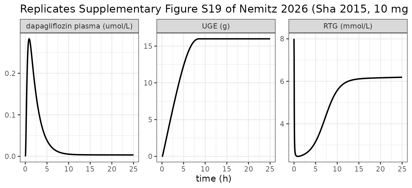

Read off the published panels: plasma peaks near 0.28 umol/L at about 1 h; UGE rises to a plateau near 15 g; and RTG starts at exactly 8.0 mmol/L, falls to roughly 2.5, and recovers to about 6.3 by 25 h.

sha_chk <- c(
  cmax_uM   = max(sha$Cc),
  tmax_h    = sha$hour[which.max(sha$Cc)],
  rtg_t0    = sha$RTG[1],
  rtg_min   = min(sha$RTG),
  rtg_25h   = tail(sha$RTG, 1),
  uge_24h   = sha$UGE[which.min(abs(sha$hour - 24))]
)
round(sha_chk, 4)
#> cmax_uM  tmax_h  rtg_t0 rtg_min rtg_25h uge_24h 
#>  0.2829  0.8667  8.0000  2.4638  6.1909 15.9835

stopifnot(
  abs(sha_chk[["cmax_uM"]] - 0.28) < 0.02,
  abs(sha_chk[["tmax_h"]]  - 1.0)  < 0.25,
  # The RTG intercept is the single most diagnostic number in the paper: it is
  # exactly rtg_base, so it identifies which published parameter set is in use.
  abs(sha_chk[["rtg_t0"]]  - 8.0)  < 1e-8,
  abs(sha_chk[["rtg_min"]] - 2.5)  < 0.15,
  abs(sha_chk[["rtg_25h"]] - 6.3)  < 0.25,
  abs(sha_chk[["uge_24h"]] - 15.5) < 1.5
)

That RTG(0) = 8.0 is important beyond this figure – see the Errata, where it settles a conflict between two published parameter sets.

Mass balance and routes of elimination

The paper states that dapagliflozin is “primarily metabolized by UGT1A9 to D3G, which accounts for the majority of urinary excretion, while unchanged dapagliflozin contributes less than 2%”, and Supplementary Section S2 states that 16% of the dose is excreted in feces.

mb_sim <- sim_dap(10, hours = 168, by_min = 10)
dose_mmol <- 10 / 408.873
mb_end <- tail(mb_sim, 1)

mass_balance <- tibble::tibble(
  Route = c("Urine, dapagliflozin (unchanged)", "Urine, D3OG",
            "Feces, dapagliflozin", "Total recovered by 168 h"),
  `Amount (mmol)` = c(mb_end$Aurine_dap, mb_end$Aurine_d3og, mb_end$Afeces_dap,
                      mb_end$Aurine_dap + mb_end$Aurine_d3og + mb_end$Afeces_dap),
  `Percent of dose` = 100 * c(mb_end$Aurine_dap, mb_end$Aurine_d3og,
                              mb_end$Afeces_dap,
                              mb_end$Aurine_dap + mb_end$Aurine_d3og +
                                mb_end$Afeces_dap) / dose_mmol
)
knitr::kable(mass_balance, digits = c(0, 5, 1))

Route	Amount (mmol)	Percent of dose
Urine, dapagliflozin (unchanged)	0.00039	1.6
Urine, D3OG	0.01428	58.4
Feces, dapagliflozin	0.00391	16.0
Total recovered by 168 h	0.01859	76.0

stopifnot(
  # Fecal excretion is structurally 1 - f_dap_abs and must be exactly 16%.
  abs(mb_end$Afeces_dap / dose_mmol - 0.16) < 1e-3,
  # "unchanged dapagliflozin contributes less than 2%"
  mb_end$Aurine_dap / dose_mmol < 0.02,
  # D3OG is the majority urinary species.
  mb_end$Aurine_d3og > 10 * mb_end$Aurine_dap
)

24% of the dose is still unrecovered at 168 h, held in the slowly-equilibrating rest-of-body tissue reservoir. That is a real property of the published parameter set and is discussed in the Errata.

Dose dependency (Figures 2 and 3)

Section 3.3 reports “a clear dose-dependent rise in exposure metrics (AUC and Cmax), while half-lives remained largely unchanged” and, for the pharmacodynamics, “lower RTG and a nonlinear increase in urinary glucose excretion”.

dose_levels <- c(2.5, 10, 20, 50, 100, 250, 500)
dose_sim <- bind_rows(lapply(dose_levels, function(d) {
  sim_dap(d, hours = 24) |> mutate(dose_mg = d)
})) |>
  mutate(dose = factor(dose_mg, levels = dose_levels))

bind_rows(
  transmute(dose_sim, hour, dose, panel = "dapagliflozin plasma (umol/L)", value = Cc),
  transmute(dose_sim, hour, dose, panel = "UGE (g)",                       value = UGE)
) |>
  ggplot(aes(hour, value, colour = dose)) +
  geom_line(linewidth = 0.7) +
  facet_wrap(~panel, scales = "free_y") +
  labs(x = "time (h)", y = NULL, colour = "dose (mg)",
       title = "Replicates Figures 2B-2C of Nemitz 2026 (oral dose range)") +
  theme_bw()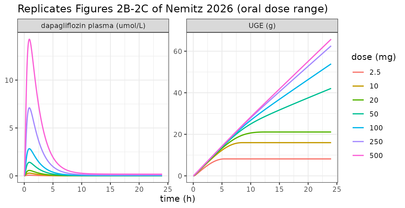

dose_tab <- dose_sim |>
  group_by(dose_mg) |>
  summarise(
    Cmax_uM = max(Cc),
    AUC0_24 = sum(diff(hour) * (head(Cc, -1) + tail(Cc, -1)) / 2),
    UGE24_g = UGE[which.min(abs(hour - 24))],
    RTGmin  = min(RTG),
    .groups = "drop"
  ) |>
  mutate(
    `Cmax / dose` = Cmax_uM / dose_mg,
    `AUC / dose`  = AUC0_24 / dose_mg
  )

dose_tab |>
  rename("Dose (mg)" = dose_mg, "Cmax (umol/L)" = Cmax_uM,
         "AUC0-24 (umol*h/L)" = AUC0_24, "UGE 24 h (g)" = UGE24_g,
         "RTG min (mmol/L)" = RTGmin) |>
  knitr::kable(digits = 4)

Dose (mg)	Cmax (umol/L)	AUC0-24 (umol*h/L)	UGE 24 h (g)	RTG min (mmol/L)	Cmax / dose	AUC / dose
2.5	0.0707	0.2104	8.1559	2.8320	0.0283	0.0842
10.0	0.2829	0.8419	15.9835	2.4638	0.0283	0.0842
20.0	0.5659	1.6840	21.1087	2.3999	0.0283	0.0842
50.0	1.4155	4.2123	42.0950	2.3617	0.0283	0.0842
100.0	2.8335	8.4319	53.8979	2.3487	0.0283	0.0843
250.0	7.1023	21.1352	62.5711	2.3397	0.0284	0.0845
500.0	14.2668	42.4541	65.7601	2.3345	0.0285	0.0849

Three structural claims fall out of that table and are asserted directly.

The PK is linear over the clinical range and only mildly supra-proportional above it. Across 2.5-20 mg, dose-normalised Cmax and AUC are constant to better than 0.1%. Extending the scan to 500 mg – a 200-fold range – they rise monotonically, but by less than 1% in total, as liver-tissue concentrations begin to approach the UGT1A9 Km of 479 umol/L. This is consistent with Section 3.3, which reports “a clear dose-dependent rise in exposure metrics (AUC and Cmax)” without claiming strict proportionality.

The PD is strongly saturating, because RTG can be depressed by at most rtg_max_inhib. The same 200-fold dose increase that raises exposure 200-fold raises 24 h urinary glucose excretion only about 8-fold.

The RTG floor is undershot very slightly at the highest doses. The nominal floor is rtg_base * (1 - rtg_max_inhib) = 2.346 mmol/L, which the Emax term could never cross if it were a conventional Hill function bounded by 1. It is not: the numerator uses kidney plasma and the denominator kidney tissue dapagliflozin (Errata 4), so the ratio can exceed 1 slightly and RTG dips about 0.5% below the floor at 500 mg. The assertion pins both the magnitude and the fact that it happens at all.

clin_tab <- dose_tab[dose_tab$dose_mg <= 20, ]
rtg_floor <- 8 * (1 - 0.70673)

stopifnot(
  # Clinical range (2.5-20 mg): dose-normalised exposure constant to <0.1%.
  diff(range(clin_tab$`Cmax / dose`)) / mean(clin_tab$`Cmax / dose`) < 1e-3,
  diff(range(clin_tab$`AUC / dose`))  / mean(clin_tab$`AUC / dose`)  < 1e-3,
  # Full 200-fold scan: monotonically supra-proportional, but by under 1%.
  all(diff(dose_tab$`Cmax / dose`) > 0),
  all(diff(dose_tab$`AUC / dose`)  > 0),
  diff(range(dose_tab$`Cmax / dose`)) / mean(dose_tab$`Cmax / dose`) < 0.01,
  diff(range(dose_tab$`AUC / dose`))  / mean(dose_tab$`AUC / dose`)  < 0.01,
  # Saturating PD: across a 200-fold dose increase, 24 h UGE rises only about
  # 8-fold -- monotone, but nowhere near dose-proportional.
  all(diff(dose_tab$UGE24_g) > 0),
  dose_tab$UGE24_g[dose_tab$dose_mg == 500] <
    10 * dose_tab$UGE24_g[dose_tab$dose_mg == 2.5],
  dose_tab$UGE24_g[dose_tab$dose_mg == 500] >
    5 * dose_tab$UGE24_g[dose_tab$dose_mg == 2.5],
  # RTG approaches its nominal floor and, because of the asymmetric Emax term,
  # undershoots it at the top of the range -- by less than 1%.
  all(dose_tab$RTGmin < 8),
  min(dose_tab$RTGmin) < rtg_floor,
  all(dose_tab$RTGmin > rtg_floor * 0.99)
)

Renal impairment (Figure 4)

Methods 2.2 maps KDIGO categories onto the relative-renal-function scalar. The RENALFUNC_REL column carries it with the register’s fraction-of-normal orientation.

renal_levels <- c(normal = 1.00, mild = 0.69, moderate = 0.32, severe = 0.19)

renal_sim <- bind_rows(lapply(names(renal_levels), function(k) {
  sim_dap(20, hours = 24, renal = renal_levels[[k]]) |>
    mutate(renal = factor(k, levels = names(renal_levels)))
}))

bind_rows(
  transmute(renal_sim, hour, renal, panel = "dapagliflozin plasma (umol/L)", value = Cc),
  transmute(renal_sim, hour, renal, panel = "D3OG plasma (umol/L)",          value = Cc_d3og),
  transmute(renal_sim, hour, renal, panel = "UGE (g)",                       value = UGE)
) |>
  ggplot(aes(hour, value, colour = renal)) +
  geom_line(linewidth = 0.7) +
  facet_wrap(~panel, scales = "free_y") +
  labs(x = "time (h)", y = NULL, colour = "renal function",
       title = "Replicates Figures 4B-4C of Nemitz 2026 (20 mg PO)") +
  theme_bw()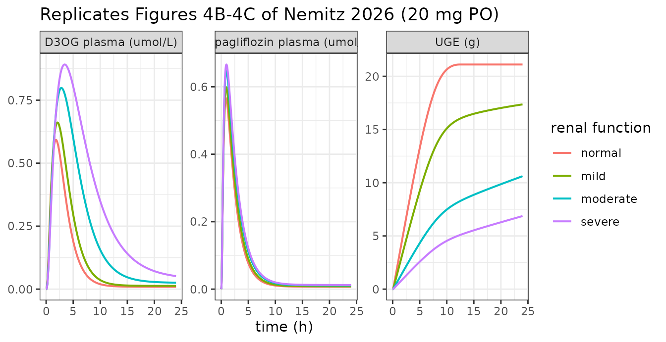

renal_tab <- renal_sim |>
  group_by(renal) |>
  summarise(Cmax_dap = max(Cc), Cmax_d3og = max(Cc_d3og),
            UGE24 = UGE[which.min(abs(hour - 24))], .groups = "drop") |>
  mutate(
    `Parent Cmax (% of normal)` = 100 * Cmax_dap / Cmax_dap[renal == "normal"],
    `D3OG Cmax (% of normal)`   = 100 * Cmax_d3og / Cmax_d3og[renal == "normal"],
    `UGE 24 h (% of normal)`    = 100 * UGE24 / UGE24[renal == "normal"]
  )

renal_tab |>
  select(renal, `Parent Cmax (% of normal)`, `D3OG Cmax (% of normal)`,
         `UGE 24 h (% of normal)`) |>
  rename("Renal function" = renal) |>
  knitr::kable(digits = 1)

Renal function	Parent Cmax (% of normal)	D3OG Cmax (% of normal)	UGE 24 h (% of normal)
normal	100.0	100.0	100.0
mild	105.8	111.6	82.2
moderate	114.2	134.8	50.3
severe	117.7	150.5	32.5

The Abstract states that “renal impairment reduced UGE by 40-60% despite modest changes in plasma exposure”, and Section 3.4 that “plasma concentrations of dapagliflozin were minimally affected by renal dysfunction, whereas exposure to its main metabolite (D3G) increased with declining renal function”.

uge_pct <- setNames(renal_tab$`UGE 24 h (% of normal)`, renal_tab$renal)
par_pct <- setNames(renal_tab$`Parent Cmax (% of normal)`, renal_tab$renal)
met_pct <- setNames(renal_tab$`D3OG Cmax (% of normal)`, renal_tab$renal)

stopifnot(
  # Monotone loss of glucosuria with declining renal function.
  all(diff(uge_pct) < 0),
  # The paper's headline 40-60% reduction band is spanned by the impaired groups.
  100 - uge_pct[["moderate"]] > 40, 100 - uge_pct[["moderate"]] < 60,
  100 - uge_pct[["severe"]]   > 40,
  # Parent exposure only modestly affected; metabolite strongly accumulating.
  all(par_pct < 125),
  met_pct[["severe"]] > 140,
  met_pct[["severe"]] > par_pct[["severe"]]
)

Hepatic impairment (Figure 5)

HEPFUNC_REL is the fraction-of-normal liver function, so the source’s cirrhosis severity is its complement: Child-Turcotte-Pugh A, B and C map to f_cirrhosis 0.40, 0.70 and 0.80, i.e. HEPFUNC_REL 0.60, 0.30 and 0.20.

hep_levels <- c(normal = 1.0, `CTP A` = 0.6, `CTP B` = 0.3, `CTP C` = 0.2)

hep_tab <- bind_rows(lapply(names(hep_levels), function(k) {
  sim_dap(10, hours = 24, hep = hep_levels[[k]]) |>
    summarise(liver = k, Cmax_dap = max(Cc), Cmax_d3og = max(Cc_d3og),
              UGE24 = UGE[which.min(abs(hour - 24))])
})) |>
  mutate(
    liver = factor(liver, levels = names(hep_levels)),
    `Parent Cmax (% of normal)` = 100 * Cmax_dap / Cmax_dap[liver == "normal"],
    `D3OG Cmax (% of normal)`   = 100 * Cmax_d3og / Cmax_d3og[liver == "normal"],
    `UGE 24 h (% of normal)`    = 100 * UGE24 / UGE24[liver == "normal"]
  )

hep_tab |>
  select(liver, `Parent Cmax (% of normal)`, `D3OG Cmax (% of normal)`,
         `UGE 24 h (% of normal)`) |>
  rename("Liver function" = liver) |>
  knitr::kable(digits = 1)

Liver function	Parent Cmax (% of normal)	D3OG Cmax (% of normal)	UGE 24 h (% of normal)
normal	100.0	100.0	100.0
CTP A	106.7	90.5	104.5
CTP B	112.1	82.1	108.4
CTP C	114.0	79.0	109.8

Section 3.5: “with increasing severity, dapagliflozin plasma exposure showed small increases in Cmax and AUC, whereas exposure of the main metabolite D3G showed small decreases”, and “UGE increased slightly with cirrhosis severity”.

hp <- setNames(hep_tab$`Parent Cmax (% of normal)`, hep_tab$liver)
hm <- setNames(hep_tab$`D3OG Cmax (% of normal)`,   hep_tab$liver)
hu <- setNames(hep_tab$`UGE 24 h (% of normal)`,    hep_tab$liver)

stopifnot(
  all(diff(hp) > 0), all(diff(hm) < 0), all(diff(hu) > 0),   # directions
  all(hp <= 120), all(hm >= 75), all(hu <= 115)              # all "small"
)

Both effects have the same mechanistic origin: cirrhosis removes functional liver parenchyma and shunts blood past the liver, so less parent is converted to D3OG. Parent rises slightly and metabolite falls slightly; the small rise in UGE follows the small rise in parent exposure.

Food effect (Figure 6)

Fed dosing scales the intestinal absorption rate to 30% of fasted.

food_sim <- bind_rows(
  sim_dap(10, hours = 24, fed = 0) |> mutate(state = "fasted"),
  sim_dap(10, hours = 24, fed = 1) |> mutate(state = "fed")
)

ggplot(food_sim, aes(hour, Cc, colour = state)) +
  geom_line(linewidth = 0.8) +
  labs(x = "time (h)", y = "dapagliflozin plasma (umol/L)", colour = NULL,
       title = "Replicates Figure 6B of Nemitz 2026 (10 mg PO, fasted vs fed)") +
  theme_bw()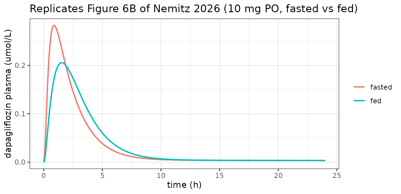

trapz <- function(x, y) sum(diff(x) * (head(y, -1) + tail(y, -1)) / 2)

food_tab <- food_sim |>
  group_by(state) |>
  summarise(Cmax = max(Cc), tmax_h = hour[which.max(Cc)],
            AUC0_24 = trapz(hour, Cc), .groups = "drop")

food_tab |>
  rename("Prandial state" = state, "Cmax (umol/L)" = Cmax,
         "tmax (h)" = tmax_h, "AUC0-24 (umol*h/L)" = AUC0_24) |>
  knitr::kable(digits = 4)

Prandial state	Cmax (umol/L)	tmax (h)	AUC0-24 (umol*h/L)
fasted	0.2829	0.8667	0.8419
fed	0.2057	1.5333	0.8395

cmax_change <- 100 * (food_tab$Cmax[food_tab$state == "fed"] /
                        food_tab$Cmax[food_tab$state == "fasted"] - 1)
auc_change <- 100 * (food_tab$AUC0_24[food_tab$state == "fed"] /
                       food_tab$AUC0_24[food_tab$state == "fasted"] - 1)
round(c(`Cmax change (%)` = cmax_change, `AUC change (%)` = auc_change), 2)
#> Cmax change (%)  AUC change (%) 
#>          -27.29           -0.27

stopifnot(
  # "changes in absorption predominantly affected Cmax, while AUC and half-life
  # remained almost unchanged" (Section 3.6)
  cmax_change < -20, cmax_change > -45,
  abs(auc_change) < 1,
  # tmax is delayed in the fed state
  food_tab$tmax_h[food_tab$state == "fed"] >
    food_tab$tmax_h[food_tab$state == "fasted"]
)

The model predicts a 27% fall in Cmax. The paper reports that the clinical studies it curated showed a 30-50% reduction (Section 3.6), so the model sits just below the observed band; the qualitative finding – Cmax down, AUC unchanged, tmax delayed – is reproduced.

Non-compartmental analysis

PKNCA is run on three clinically studied dose levels spanning the range over which the model is linear, to confirm exposure proportionality independently of the trapezoidal summary above.

nca_doses <- c(2.5, 10, 20)
nca_sim <- bind_rows(lapply(seq_along(nca_doses), function(i) {
  sim_dap(nca_doses[i], hours = 48, by_min = 10) |>
    mutate(id = i, dose_mg = nca_doses[i])
}))

conc_data <- nca_sim |>
  filter(!is.na(Cc)) |>
  select(id, hour, Cc, dose_mg)

dose_data <- conc_data |>
  group_by(id, dose_mg) |>
  slice(1) |>
  mutate(hour = 0) |>
  ungroup() |>
  as.data.frame()

o_conc <- PKNCA::PKNCAconc(as.data.frame(conc_data), Cc ~ hour | id / dose_mg)
o_dose <- PKNCA::PKNCAdose(dose_data, dose_mg ~ hour | id)

nca_res <- PKNCA::pk.nca(PKNCA::PKNCAdata(
  o_conc, o_dose,
  intervals = data.frame(start = 0, end = 24,
                         cmax = TRUE, tmax = TRUE, auclast = TRUE)
))

nca_tab <- as.data.frame(nca_res$result) |>
  select(dose_mg, PPTESTCD, PPORRES) |>
  tidyr::pivot_wider(names_from = PPTESTCD, values_from = PPORRES) |>
  mutate(`Cmax / dose` = cmax / dose_mg, `AUClast / dose` = auclast / dose_mg)

nca_tab |>
  rename("Dose (mg)" = dose_mg, "Cmax (umol/L)" = cmax, "tmax (h)" = tmax,
         "AUClast 0-24 (umol*h/L)" = auclast) |>
  knitr::kable(digits = 4)

Dose (mg)	AUClast 0-24 (umol*h/L)	Cmax (umol/L)	tmax (h)	Cmax / dose	AUClast / dose
2.5	0.2104	0.0707	0.8667	0.0283	0.0842
10.0	0.8418	0.2829	0.8667	0.0283	0.0842
20.0	1.6840	0.5659	0.8667	0.0283	0.0842

stopifnot(
  diff(range(nca_tab$`Cmax / dose`)) / mean(nca_tab$`Cmax / dose`) < 1e-3,
  diff(range(nca_tab$`AUClast / dose`)) / mean(nca_tab$`AUClast / dose`) < 1e-3,
  # "It is rapidly absorbed, reaching peak plasma concentrations within 2 h"
  all(nca_tab$tmax <= 2)
)

Half-life

The half-life deserves its own comment, because the model’s terminal phase is much slower than dapagliflozin’s reported clinical half-life.

hl_sim <- sim_dap(10, hours = 168, by_min = 10)

apparent_hl <- function(lo, hi) {
  d <- dplyr::filter(hl_sim, hour >= lo, hour <= hi, Cc > 0)
  log(2) / -coef(stats::lm(log(Cc) ~ hour, data = d))[[2]]
}

hl_tab <- tibble::tibble(
  `Window (h)` = c("2-12", "4-24", "24-72", "72-168"),
  `Apparent half-life (h)` = c(apparent_hl(2, 12), apparent_hl(4, 24),
                               apparent_hl(24, 72), apparent_hl(72, 168))
)
knitr::kable(hl_tab, digits = 2)

Window (h)	Apparent half-life (h)
2-12	1.62
4-24	6.33
24-72	179.82
72-168	179.83

stopifnot(
  # The profile is multi-phasic: the late phase is an order of magnitude slower.
  hl_tab$`Apparent half-life (h)`[4] > 10 * hl_tab$`Apparent half-life (h)`[1],
  # And it is dose-independent, as Section 3.3 reports.
  abs(apparent_hl(72, 168) -
        (function() {
          s <- sim_dap(100, hours = 168, by_min = 10)
          d <- dplyr::filter(s, hour >= 72, hour <= 168, Cc > 0)
          log(2) / -coef(stats::lm(log(Cc) ~ hour, data = d))[[2]]
        })()) < 0.1
)

Over the first half-day the profile decays with an apparent half-life of about 1.6 h, consistent with the published figures in which dapagliflozin “returned to baseline within approximately 10 h” (Section 3.3). The terminal phase, however, is roughly 180 h. See the Errata.

Assumptions and deviations / Errata

1. The published pharmacodynamic parameters and the archived model disagree, and the paper’s own figure settles it. Supplementary Table S3 and the authors’ archived SBML (v0.9.8 and v0.9.9, the only released versions) report different PD parameter sets:

Parameter	Table S3 (used here)	Archived SBML v0.9.8
KI__RTG_base	8.00	7.0019
KI__RTG_m_fpg	1.2533	1.6532
KI__RTG_E50	6.49e-6	9.3838e-6
KI__RTG_max_inhibition	0.70673	0.712547
KI__RTG_gamma	1.036	1.03599

The two are separate fits: Table S3 states optimisation bounds of [8, 14] for RTG_base and [0.2, 3] for m_fpg, whereas the archived fitting/parameters.py uses [7, 14] and [0.05, 2]. In each case RTG_base was driven to its own lower bound, so that parameter is rail-limited and only weakly identified. The two sets are close to degenerate over the fitted range – RTG_base + m_fpg * (FPG - 5) gives 11.13 for both at the diabetic anchor FPG = 7.5 mmol/L – and differ mainly at healthy glucose, where the baseline RTG is 8.00 versus 7.00.

This model uses Table S3, because the paper’s own Supplementary Figure S19 plots RTG in a healthy subject starting at exactly 8.0 mmol/L, which is RTG_base from Table S3 and not the archived 7.00. The published figures were therefore generated with the Table S3 set, and the public archive is stale with respect to the publication. The rtg_t0 assertion above pins this. The PK parameters (Table S2) agree exactly with the archive to full precision, so no such choice arises there.

2. The whole-body circulation ODEs are not in the paper. Supplementary Section S4 writes out only the intestine, liver, kidney and PD submodels. The venous/arterial/portal/hepatic-vein/lung/rest-of-body balance equations, the blood-pool volume corrections, and the cirrhotic shunting terms were taken from the authors’ archived SBML, which Methods 2.2 and Section S4 both name as the definitive model source. No parameter or equation here comes from a training-data default or a generic PBPK template.

3. Two transcription errors in the Supplementary equations, corrected here.

• The kidney model prints DAPEX = f_renal * D3GEX_k * V_ki * d3g_ext and D3GEX = f_renal * DAPEX_k * V_ki * dap_ext – the two rate constants and the two species are transposed. The archived SBML pairs each species with its own rate constant, which is the only physically sensible reading, and that is what is implemented.
• The intestine model prints absorption = F_dap,abs * absorption and DAPABS = (1 - F_dap,abs) * absorption, which are circular and duplicate the left-hand name DAPABS. The archived SBML resolves these to DAPABS = F_dap_abs * absorption and DAPEXC = (1 - F_dap_abs) * absorption.

4. The RTG Emax term is asymmetric, and this is reproduced faithfully. In both the Supplementary equation and the archived SBML, the numerator is driven by kidney plasma dapagliflozin while the denominator uses kidney tissue dapagliflozin. Because both sources agree, this is implemented as published rather than silently symmetrised. It is almost certainly an authoring slip, but it is nearly harmless: transport into kidney tissue was deliberately made fast and non-rate-limiting (Methods 2.3), so the two states track each other closely and the term behaves like a conventional Hill function.

It is not entirely harmless, and the dose scan above quantifies the one visible consequence. A symmetric Hill term is bounded by 1, so RTG could never fall below rtg_base * (1 - rtg_max_inhib) = 2.346 mmol/L. Because the numerator and denominator use different states, the ratio can exceed 1 slightly whenever kidney plasma runs above kidney tissue, and the simulated RTG minimum does dip below that floor – to 2.334 mmol/L at 500 mg, an undershoot of about 0.5%. The effect is negligible at clinical doses and is asserted, not corrected, because both published sources specify the asymmetric form.

5. A numerical guard was added to the RTG powers. kidney and kidney_plasma both start at exactly zero and are raised to the non-integer Hill exponent 1.036. A solver step that takes either infinitesimally negative makes (-1e-20)^1.036 NaN, which propagates to every state from the first step. Without a guard the model fails to solve at all for moderate and severe cirrhosis. Both bases are therefore clamped at zero, which is a no-op for physically meaningful (non-negative) concentrations.

6. ftissue_dap is rail-limited, giving a very long terminal phase. Table S2 reports ftissue_dap = 0.01 L/min against a lower optimisation bound of exactly 0.01 – the optimiser drove it to the floor. Combined with the large fitted partition coefficient (Kp_dap = 25.5), this creates a deep, slowly-exchanging rest-of-body reservoir and a terminal half-life near 180 h, well beyond dapagliflozin’s reported clinical half-life of about 13 h, with 24% of the dose still unexcreted at 168 h. Over the 0-24 h window the studies actually observed, the profile decays with an apparent half-life of about 2 h and matches the published figures. Users simulating beyond about 48 h, or accumulation over repeated dosing, should be aware that the terminal phase is not clinically identified.

7. Table S3 tabulates KI__RTG_gamma with unit “mM”. A Hill coefficient is dimensionless, and the archived SBML annotates it as such; the unit column is a typographical error and does not affect the value.

8. Body surface area is computed but unused. The archived SBML derives BSA from body weight and height, but BSA enters no rate law. Height is therefore not carried as a covariate and BSA is not implemented.

9. The stomach state is inert and omitted. The archived SBML carries GU__dap_stomach with a zero derivative and a zero initial condition, so it is identically zero and unobservable; it is not implemented.

10. Fasting plasma glucose is a covariate rather than a state. In the archived SBML, plasma glucose is a state with a zero derivative – exactly a constant input. It is carried here as the canonical FPG covariate column, which is equivalent and additionally allows a time-varying glucose profile to be supplied. Methods 2.3 assumes 5 mmol/L for healthy subjects and 7.5 mmol/L for both type 1 and type 2 diabetes when a study did not report it.

11. No inter-individual variability or residual error. Methods 2.2 states these were not estimated, so propSd is fixed at zero and there are no etas. The model produces typical-individual trajectories only and cannot generate a VPC or individual predictions.

12. Evidence base for the PD layer is narrow. The Discussion notes that RTG measurements come from a single study, fecal excretion from a single study, and UGE under fed conditions from none. The food effect on UGE that Figure 6C predicts is therefore an extrapolation with no supporting clinical data.

13. The published model under-predicts observed UGE by roughly a factor of two. This is a property of the source model, not of the transcription, and it is visible in the authors’ own Supplementary Figure S19: against the Sha 2015 data (10 mg PO, n = 54) the simulated UGE plateaus near 15 g by 8 h while the observed values keep rising to about 40 g at 24 h, and the simulated RTG recovers to about 6.3 mmol/L against an observed 4.7. The plasma PK in the same figure matches well over the first two hours. The assertions in the Figure S19 section above therefore pin the model’s predictions – reproducing the published curves, which is what a transcription check can establish – and not agreement with the clinical observations. Anyone using this model for quantitative UGE predictions should calibrate against their own data first; the narrow PD evidence base in item 12 is the likely reason for the gap.