Model and source
- Citation: Nava T, Kassir N, Rezgui MA, Uppugunduri CRS, Huezo-Diaz Curtis P, Duval M, Theoret Y, Daudt LE, Litalien C, Ansari M, Krajinovic M, Bittencourt H. Incorporation of GSTA1 genetic variations into a population pharmacokinetic model for IV busulfan in paediatric hematopoietic stem cell transplantation. Br J Clin Pharmacol. 2018;84(7):1494-1504. doi:10.1111/bcp.13566. The maturation function is Equation D of the paper’s Supplemental Material Table S2, which reproduces McCune JS, Bemer MJ, Barrett JS, Scott Baker K, Gamis AS, Holford NH. Clin Cancer Res 2014;20(3):754-763. doi:10.1158/1078-0432.CCR-13-1960.
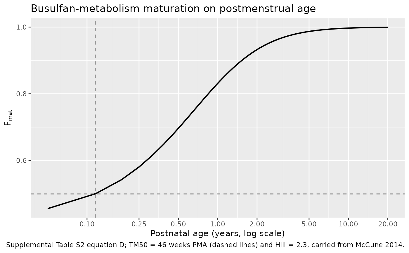
- Description: One-compartment IV population PK model with first-order elimination for intravenous busulfan in children and adolescents (0.1-20 years) undergoing conditioning before haematopoietic stem cell transplantation. Theory-based allometric scaling of actual body weight (exponent 0.75 on CL, 1 on V) referenced to 70 kg; a sigmoid Emax maturation function of postmenstrual age on clearance carried over unchanged from McCune 2014 (TM50 = 46 weeks, Hill = 2.3); a power effect of postmenstrual age on volume; and a three-level GSTA1 diplotype effect on clearance (rapid metabolizers 7% faster, poor metabolizers 12% slower than normal metabolizers). Between-subject variability on CL and V, between-occasion variability on CL and V across the four days of busulfan dosing, and a proportional residual error. This is the first paediatric busulfan popPK model to incorporate a pharmacogenetic covariate (Nava 2018).
- Article: https://doi.org/10.1111/bcp.13566
- Supplement (Tables S1-S6, Figures S1-S5, and the maturation / size
equations used in the model): https://pmc.ncbi.nlm.nih.gov/articles/PMC6005620/
(Supporting Information file
BCP-84-1494-s001.docx). Every value this vignette attributes to the supplement was read from that file directly; the quoted Table S2 row labels below are verbatim.
Nava 2018 is the first paediatric population PK model for intravenous busulfan to carry a pharmacogenetic covariate. Busulfan is conjugated to glutathione by glutathione S-transferase A1, and promoter variants of GSTA1 change how much enzyme is expressed. The authors genotyped four GSTA1 promoter loci, built diplotypes from them, and grouped patients into rapid (G1), normal (G2) and poor (G3) metabolizers. Group membership turned out to be a significant covariate on busulfan clearance, and adding it cut the unexplained between-subject variability in clearance by 27%.
Population
The model was built from 199 PK profiles and 1735 plasma busulfan concentrations contributed by 112 children and adolescents (median 5.4 years, range 0.1-20) conditioned for autologous or allogeneic haematopoietic stem cell transplantation at CHU Sainte-Justine (Montreal) between April 2002 and August 2016 (Nava 2018 Table 1 and Results). 52.7% were female; 83.9% Caucasian, 10.7% African and 5.4% other; 66.1% had a malignant diagnosis. GSTA1 diplotype groups were G1 14.3%, G2 71.4% and G3 14.3%.
Two dosing schedules are represented. Until April 2012 busulfan was given as a 2-h infusion every 6 h (Bu6); from May 2012 as a 3-h infusion every 24 h (Bu24) at four times the corresponding Bu6 dose. Both run for four consecutive days. Regimens in which another chemotherapeutic drug was given before or during the busulfan infusion days were excluded, so that fludarabine-associated clearance changes could not bias the fit.
Nava 2018 Table 1 reports no body-weight summary – only weight adequacy (12.5% overweight, 6.3% obese among children older than 2 years) – so the virtual cohort below derives weight from age; see “Assumptions and deviations”.
The same information is available programmatically via the model’s
population metadata:
pop <- rxode2::rxode(readModelDb("Nava_2018_busulfan"))$population
#> ℹ parameter labels from comments will be replaced by 'label()'
#> Warning: some etas defaulted to non-mu referenced, possible parsing error: etaiov_cl_1, etaiov_cl_2, etaiov_cl_3, etaiov_cl_4, etaiov_vc_1, etaiov_vc_2, etaiov_vc_3, etaiov_vc_4
#> as a work-around try putting the mu-referenced expression on a simple line
str(pop, max.level = 1)
#> List of 11
#>  $ species       : chr "human"
#>  $ n_subjects    : int 112
#>  $ n_studies     : int 1
#>  $ age_range     : chr "0.1-20 years"
#>  $ age_median    : chr "5.4 years"
#>  $ sex_female_pct: num 52.7
#>  $ race_ethnicity: Named num [1:3] 83.9 10.7 5.4
#>   ..- attr(*, "names")= chr [1:3] "Caucasian" "African" "Other"
#>  $ disease_state : chr "Children and adolescents receiving intravenous busulfan as part of the conditioning regimen before autologous o"| __truncated__
#>  $ dose_range    : chr "Intravenous busulfan for four consecutive days on one of two schedules. Bu6 (April 2002 - April 2012): 2-h infu"| __truncated__
#>  $ regions       : chr "Canada (single centre: CHU Sainte-Justine, Montreal, Quebec)"
#>  $ notes         : chr "Retrospective chart review of paediatric transplants performed between April 2002 and August 2016; part of NCT0"| __truncated__
Source trace
The per-parameter origin is recorded as an in-file comment next to
each ini() entry in
inst/modeldb/specificDrugs/Nava_2018_busulfan.R. The table
below collects them in one place.
| Equation / parameter | Value | Source location |
|---|---|---|
lcl (CL at 70 kg) |
13.70 L/h | Table 2, Final model (RSE 2.43%); also the displayed clearance equation, p. 1497 |
lvc (V at 70 kg) |
49.57 L | Table 2, Final model (RSE 1.15%) |
e_wt_cl |
0.75 (fixed) | Displayed clearance equation, p. 1497:
CL = 13.7 * (ABW/70)^0.75 * Fmat * F_GSTA1; Supplemental
Table S2 equation C row label |
e_wt_vc |
1 (fixed) | Supplemental Table S2, equation C row label
Fsize, where pwr = 1 for V and 0.75 for CL; Results, “Base
model” – “theoretical allometric scaling of the actual body weight
(ABW)” |
tm50_mat |
46 weeks (fixed) | Supplemental Table S2, row label
Fmat, where TM50=46; Hill's coefficient=2.3; restated in
Discussion, p. 1499 |
hill_mat |
2.3 (fixed) | Supplemental Table S2, same row label |
e_page_vc |
-0.06 | Table 2, Final model, “PMA on V” (RSE 23.40%) |
pma_ref |
320.8 weeks (fixed) |
Not printed. Derived from Table 1 median age 5.4 y
via Supplemental Table S2 equation E (PMA = 52 * AGE + 40);
see “Assumptions and deviations” |
e_gsta1_rm_cl |
1.07 | Table 2, Final model, G1 (RSE 4.40%); p. 1497 “F_GSTA1
= 1.07 for G1” |
e_gsta1_pm_cl |
0.88 | Table 2, Final model, G3 (RSE 0.40%); p. 1497 “0.88 for G3 patients” |
etalcl (BSV CL) |
13.30% CV | Table 2, Final model (RSE 8.80%, shrinkage 6.00%); restated in Discussion, p. 1500 |
etalvc (BSV V) |
7.00% CV | Table 2, Final model (RSE 19.20%, shrinkage 24.60%); restated in Discussion, p. 1500 |
etaiov_cl_* (BOV CL) |
7.30% CV | Table 2, Final model (RSE 8.10%, shrinkage 46.60%) |
etaiov_vc_* (BOV V) |
9.60% CV | Table 2, Final model (RSE 16.40%, shrinkage 9.30%) |
propSd |
7.40% | Table 2, Final model, sigma [Proportional error (%)] (RSE 7.90%) |
Fmat = 1 / (1 + (PMA/TM50)^-Hill) |
n/a | Supplemental Table S2 equation D (reproducing McCune 2014) |
PMA[weeks] = 52 * AGE[years] + 40 |
n/a | Supplemental Table S2 equation E |
d/dt(central) = -kel * central |
n/a | Results, “Base model” – one-compartment model with first-order elimination |
| AUC unit conversion 0.0041 | n/a | Supplemental Table S3 footnote a |
| Target AUC windows | 3600-6000 / 900-1500 uM.min | Methods, “Comparison with other available PopPK models”; Table 3 heading |
Unit conventions and their internal consistency
Busulfan exposure is conventionally reported in uM.min while the model works in mg/L and hours. The paper states the conversion three separate ways, and all three agree with the molecular weight of busulfan (246.29 g/mol). Reproducing that agreement is the cheapest possible check that the exposure targets used below are on the model’s scale.
mw_busulfan <- 246.29  # g/mol

# 1 uM.min expressed in mg*h/L.
uMmin_to_mghL <- mw_busulfan / 1000 / 60

# Supplemental Table S3 footnote a: "0.0041 is the conversion factor to convert
# the AUC units from uM.min/L to mg.h/L".
stopifnot(abs(uMmin_to_mghL - 0.0041) < 0.00005)

# Supplemental Table S3 footnote b: "4.72 mg/h/L = 1150 uM.min".
stopifnot(abs(1150 * uMmin_to_mghL - 4.72) < 0.01)

# Methods: a target Css of 0.77 mg/L is "equivalent to AUC24h of 4500 uM min
# or AUC6h of 1125 uM min".
css_target_mgL <- 0.77
stopifnot(
  abs(css_target_mgL * 24 / uMmin_to_mghL - 4500) < 25,
  abs(css_target_mgL *  6 / uMmin_to_mghL - 1125) < 10
)

auc24_target_mghL <- 4500 * uMmin_to_mghL
auc6_target_mghL  <- 1125 * uMmin_to_mghL
auc24_window_mghL <- c(3600, 6000) * uMmin_to_mghL
auc6_window_mghL  <- c( 900, 1500) * uMmin_to_mghL

# Methods, "Treatment regimen": PK-guided dose adjustment aimed "for a total
# cumulative AUC of 18 000 uM min every 4 days". Over four days the Bu24
# schedule delivers 4 doses at the AUC24h target and the Bu6 schedule delivers
# 16 doses at the AUC6h target, and both arrive at the same cumulative figure --
# and at the same cumulative therapeutic window. That the paper's per-interval
# and cumulative numbers agree exactly is a check on the transcription of all
# five of them.
stopifnot(
  4 * 4500 == 18000,
  16 * 1125 == 18000,
  all(4 * c(3600, 6000) == 16 * c(900, 1500))
)

auc_cum_target_mghL <- 18000 * uMmin_to_mghL
auc_cum_window_mghL <- 4 * c(3600, 6000) * uMmin_to_mghL

tibble::tibble(
  Quantity = c("1 uM.min", "AUC24h target 4500 uM.min",
               "AUC24h window 3600-6000 uM.min",
               "AUC6h target 1125 uM.min",
               "AUC6h window 900-1500 uM.min"),
  `mg*h/L` = c(
    sprintf("%.6f", uMmin_to_mghL),
    sprintf("%.2f", auc24_target_mghL),
    sprintf("%.2f-%.2f", auc24_window_mghL[1], auc24_window_mghL[2]),
    sprintf("%.2f", auc6_target_mghL),
    sprintf("%.2f-%.2f", auc6_window_mghL[1], auc6_window_mghL[2])
  )
) |>
knitr::kable(caption = "Busulfan exposure units, from the paper's own conversion factors.")| Quantity | mg*h/L |
|---|---|
| 1 uM.min | 0.004105 |
| AUC24h target 4500 uM.min | 18.47 |
| AUC24h window 3600-6000 uM.min | 14.78-24.63 |
| AUC6h target 1125 uM.min | 4.62 |
| AUC6h window 900-1500 uM.min | 3.69-6.16 |
Replicating the published clearance equation
Nava 2018 prints its individualized clearance on p. 1497:
with F_GSTA1 = 1.07 (G1), 1 (G2), 0.88 (G3), and
Fmat = 1 / (1 + (PMA/46)^-2.3) from Supplemental Table S2
equation D. The check below evaluates that expression independently in R
and compares it with the clearance the packaged model computes for the
same subject. This is a deterministic comparison – both sides use the
same fixed parameters and no random effects – so the tolerance is
tight.
mod_ui  <- rxode2::rxode(readModelDb("Nava_2018_busulfan"))
#> ℹ parameter labels from comments will be replaced by 'label()'
#> Warning: some etas defaulted to non-mu referenced, possible parsing error: etaiov_cl_1, etaiov_cl_2, etaiov_cl_3, etaiov_cl_4, etaiov_vc_1, etaiov_vc_2, etaiov_vc_3, etaiov_vc_4
#> as a work-around try putting the mu-referenced expression on a simple line
mod_typ <- rxode2::zeroRe(mod_ui)
#> Warning: some etas defaulted to non-mu referenced, possible parsing error: etaiov_cl_1, etaiov_cl_2, etaiov_cl_3, etaiov_cl_4, etaiov_vc_1, etaiov_vc_2, etaiov_vc_3, etaiov_vc_4
#> as a work-around try putting the mu-referenced expression on a simple line

pma_from_age <- function(age_years) 52 * age_years + 40  # Suppl. Table S2 eq. E

# The paper's equation, transcribed directly.
cl_paper <- function(abw, age_years, gsta1_group) {
  pma   <- pma_from_age(age_years)
  fmat  <- 1 / (1 + (pma / 46)^(-2.3))
  fgst  <- c(G1 = 1.07, G2 = 1.00, G3 = 0.88)[gsta1_group]
  unname(13.7 * (abw / 70)^0.75 * fmat * fgst)
}

probe <- tidyr::expand_grid(
  age_years   = c(0.1, 0.5, 1, 2, 5.4, 10, 16, 20),
  gsta1_group = c("G1", "G2", "G3")
) |>
  mutate(
    WT       = c(4.5, 7.6, 9.6, 12.2, 19.5, 32.0, 57.5, 65.0)[
      match(age_years, c(0.1, 0.5, 1, 2, 5.4, 10, 16, 20))],
    PAGE     = pma_from_age(age_years),
    GSTA1_RM = as.integer(gsta1_group == "G1"),
    GSTA1_PM = as.integer(gsta1_group == "G3"),
    OCC      = 1L,
    id       = row_number()
  )

# A single dose plus one observation is enough to make rxode2 report `cl`.
probe_ev <- bind_rows(
  probe |> mutate(time = 0, evid = 1L, amt = 1, dur = 1, cmt = "central"),
  probe |> mutate(time = 2, evid = 0L, amt = NA_real_, dur = NA_real_,
                  cmt = "central")
) |>
  arrange(id, time, desc(evid))

probe_sim <- rxode2::rxSolve(
  mod_typ, probe_ev,
  keep = c("gsta1_group", "age_years"),
  covsInterpolation = "locf", useLinCmt = FALSE,
  returnType = "data.frame"
)
#> ℹ omega/sigma items treated as zero: 'etalcl', 'etalvc', 'etaiov_cl_1', 'etaiov_cl_2', 'etaiov_cl_3', 'etaiov_cl_4', 'etaiov_vc_1', 'etaiov_vc_2', 'etaiov_vc_3', 'etaiov_vc_4'
#> Warning: multi-subject simulation without without 'omega'

cl_chk <- probe_sim |>
  group_by(id, gsta1_group, age_years) |>
  summarise(cl_model = first(cl), .groups = "drop") |>
  left_join(probe |> select(id, WT), by = "id") |>
  mutate(
    cl_equation = cl_paper(WT, age_years, gsta1_group),
    pct_diff    = 100 * (cl_model - cl_equation) / cl_equation
  )

# Deterministic: same fixed parameters on both sides, no random effects, so the
# only difference possible is numerical round-off.
stopifnot(max(abs(cl_chk$pct_diff)) < 1e-6)

cl_chk |>
  filter(gsta1_group == "G2") |>
  transmute(
    `Age (years)`        = age_years,
    `Weight (kg)`        = WT,
    `PMA (weeks)`        = pma_from_age(age_years),
    `Fmat`               = round(1 / (1 + (pma_from_age(age_years) / 46)^(-2.3)), 4),
    `CL, paper eq (L/h)` = round(cl_equation, 3),
    `CL, model (L/h)`    = round(cl_model, 3)
  ) |>
  knitr::kable(
    digits  = 3,
    caption = "Model clearance vs the p. 1497 equation, normal metabolizers (G2)."
)| Age (years) | Weight (kg) | PMA (weeks) | Fmat | CL, paper eq (L/h) | CL, model (L/h) |
|---|---|---|---|---|---|
| 0.1 | 4.5 | 45.2 | 0.490 | 0.857 | 0.857 |
| 0.5 | 7.6 | 66.0 | 0.696 | 1.805 | 1.805 |
| 1.0 | 9.6 | 92.0 | 0.831 | 2.566 | 2.566 |
| 2.0 | 12.2 | 144.0 | 0.932 | 3.446 | 3.446 |
| 5.4 | 19.5 | 320.8 | 0.989 | 5.194 | 5.194 |
| 10.0 | 32.0 | 560.0 | 0.997 | 7.592 | 7.592 |
| 16.0 | 57.5 | 872.0 | 0.999 | 11.807 | 11.807 |
| 20.0 | 65.0 | 1080.0 | 0.999 | 12.950 | 12.950 |
The GSTA1 effect is a pure multiplier on clearance, so the ratios reproduce the abstract’s “7% faster in rapid metabolizers and 12% slower in poor metabolizers”.
# Pivot on age_years, not id: `id` is unique per (age, GSTA1 group) pair, so
# pivoting on it would put each group in its own row and leave the other two
# columns NA.
gsta1_ratio <- cl_chk |>
  select(age_years, gsta1_group, cl_model) |>
  tidyr::pivot_wider(names_from = gsta1_group, values_from = cl_model) |>
  mutate(ratio_G1 = G1 / G2, ratio_G3 = G3 / G2)

stopifnot(nrow(gsta1_ratio) == dplyr::n_distinct(cl_chk$age_years),
          !anyNA(gsta1_ratio))

stopifnot(
  max(abs(gsta1_ratio$ratio_G1 - 1.07)) < 1e-6,
  max(abs(gsta1_ratio$ratio_G3 - 0.88)) < 1e-6
)

c(`G1 / G2` = unique(round(gsta1_ratio$ratio_G1, 4)),
  `G3 / G2` = unique(round(gsta1_ratio$ratio_G3, 4)))
#> G1 / G2 G3 / G2
#>    1.07    0.88
Maturation and size over the paediatric age range
mat_curve <- tibble::tibble(age_years = seq(0.05, 20, length.out = 300)) |>
  mutate(
    PAGE = pma_from_age(age_years),
    Fmat = 1 / (1 + (PAGE / 46)^(-2.3))
  )

ggplot(mat_curve, aes(age_years, Fmat)) +
  geom_line(linewidth = 0.8) +
  geom_hline(yintercept = 0.5, linetype = "dashed", colour = "grey40") +
  geom_vline(xintercept = (46 - 40) / 52, linetype = "dashed", colour = "grey40") +
  scale_x_log10(breaks = c(0.1, 0.25, 0.5, 1, 2, 5, 10, 20)) +
  labs(
    x = "Postnatal age (years, log scale)",
    y = expression(F[mat]),
    title = "Busulfan-metabolism maturation on postmenstrual age",
    caption = paste(
      "Supplemental Table S2 equation D; TM50 = 46 weeks PMA (dashed lines)",
      "and Hill = 2.3, carried from McCune 2014."
    )
  )
Virtual cohort
Original observed data are not publicly available. The cohort below approximates the published demographics: median age 5.4 years over a 0.1-20 year range (Table 1), GSTA1 groups 14.3% / 71.4% / 14.3%, and weight derived from age because the paper reports none.
# `set.seed()` seeds R's RNG. It does NOT seed rxode2's simulation RNG, and
# rxode2's streams are partitioned per solver thread, so the sampled etas differ
# between a 2-thread CI runner and a 16-thread workstation. Every assertion
# downstream is written to hold for any cohort this model can produce.
set.seed(20180209)

n_subj <- 200

# Age: log-normal centred on the Table 1 median of 5.4 years, truncated to the
# reported 0.1-20 year range.
age_years <- pmin(pmax(exp(rnorm(n_subj, log(5.4), 1.0)), 0.1), 20)

# Weight-for-age. Nava 2018 reports no weights, so the cohort uses approximate
# 50th-percentile CDC weight-for-age (sexes pooled) with 15% CV log-normal
# scatter. See "Assumptions and deviations".
wfa_age <- c(0, 0.25, 0.5, 1, 2, 3, 4, 6, 8, 10, 12, 14, 16, 18, 20)
wfa_kg  <- c(3.4, 6.0, 7.6, 9.6, 12.2, 14.3, 16.3, 20.8, 25.8,
             32.0, 40.5, 50.0, 57.5, 62.0, 65.0)
wt_median <- stats::approx(wfa_age, wfa_kg, xout = age_years, rule = 2)$y
WT <- pmax(wt_median * exp(rnorm(n_subj, 0, 0.15)), 2.5)

# GSTA1 diplotype group per Table 1.
gsta1_group <- sample(c("G1", "G2", "G3"), n_subj, replace = TRUE,
                      prob = c(0.143, 0.714, 0.143))

cohort <- tibble::tibble(
  id          = seq_len(n_subj),
  age_years   = age_years,
  WT          = WT,
  PAGE        = pma_from_age(age_years),
  gsta1_group = gsta1_group,
  GSTA1_RM    = as.integer(gsta1_group == "G1"),
  GSTA1_PM    = as.integer(gsta1_group == "G3")
)

cohort |>
  summarise(
    n            = n(),
    `Age median` = round(median(age_years), 2),
    `Age min`    = round(min(age_years), 2),
    `Age max`    = round(max(age_years), 2),
    `WT median`  = round(median(WT), 1),
    `% G1`       = round(100 * mean(GSTA1_RM), 1),
    `% G3`       = round(100 * mean(GSTA1_PM), 1)
  ) |>
knitr::kable(caption = "Virtual cohort (target: median age 5.4 y, 14.3% G1, 14.3% G3).")| n | Age median | Age min | Age max | WT median | % G1 | % G3 |
|---|---|---|---|---|---|---|
| 200 | 5.04 | 0.24 | 20 | 19.5 | 13.5 | 11 |
Simulation
The paper’s dose-selection logic is “estimate the first dose from the
model-predicted individual clearance and the target AUC” (Methods,
“Comparison with other available PopPK models”):
Dose = AUC_target x CL. A first dose is chosen before any
concentration has been measured, so the clearance available at that
moment is the population prediction for the subject’s
covariates – no random effects. Each subject then receives that dose and
is simulated with the full between-subject and between-occasion
variability.
Both schedules are simulated as separate arms with disjoint subject IDs.
# Population-predicted clearance (no random effects) for dose selection.
dose_probe_ev <- bind_rows(
  cohort |> mutate(time = 0, evid = 1L, amt = 1, dur = 1, cmt = "central",
                   OCC = 1L),
  cohort |> mutate(time = 2, evid = 0L, amt = NA_real_, dur = NA_real_,
                   cmt = "central", OCC = 1L)
) |>
  arrange(id, time, desc(evid))

cl_pop <- rxode2::rxSolve(
  mod_typ, dose_probe_ev,
  covsInterpolation = "locf", useLinCmt = FALSE, returnType = "data.frame"
) |>
  group_by(id) |>
  summarise(cl_pop = first(cl), .groups = "drop")
#> ℹ omega/sigma items treated as zero: 'etalcl', 'etalvc', 'etaiov_cl_1', 'etaiov_cl_2', 'etaiov_cl_3', 'etaiov_cl_4', 'etaiov_vc_1', 'etaiov_vc_2', 'etaiov_vc_3', 'etaiov_vc_4'
#> Warning: multi-subject simulation without without 'omega'

cohort_dosed <- cohort |>
  left_join(cl_pop, by = "id") |>
  mutate(
    dose_bu24_mg = auc24_target_mghL * cl_pop,
    dose_bu6_mg  = auc6_target_mghL  * cl_pop
  )

# Observation grids: fine over the first dosing interval (where the NCA is
# taken), coarse afterwards so the four-day profile can still be plotted.
grid_bu24 <- sort(unique(c(seq(0, 24, by = 0.25), seq(25, 96, by = 1))))
grid_bu6  <- sort(unique(c(seq(0, 6,  by = 0.10), seq(6.5, 96, by = 0.5))))

# Occasion = busulfan dosing day, 1-4 (see the model's covariateData$OCC).
occ_for_time <- function(tm) pmin(pmax(floor(tm / 24) + 1L, 1L), 4L)

build_arm <- function(dose_mg, dur_h, ii_h, addl, obs_grid, regimen,
                      id_offset = 0L) {
  covs <- cohort_dosed |>
    mutate(id = id + id_offset, amt_mg = dose_mg) |>
    select(id, WT, PAGE, GSTA1_RM, GSTA1_PM, gsta1_group, amt_mg)

  doses <- tidyr::expand_grid(
    covs, time = seq(0, by = ii_h, length.out = addl + 1L)
  ) |>
    mutate(evid = 1L, amt = amt_mg, dur = dur_h, cmt = "central", ii = 0,
           addl = 0L)

  obs <- tidyr::expand_grid(covs, time = obs_grid) |>
    mutate(evid = 0L, amt = NA_real_, dur = NA_real_, cmt = "central",
           ii = 0, addl = 0L)

  bind_rows(doses, obs) |>
    mutate(OCC = occ_for_time(time), regimen = regimen) |>
    arrange(id, time, desc(evid))
}

events <- bind_rows(
  build_arm(cohort_dosed$dose_bu24_mg, dur_h = 3, ii_h = 24, addl = 3L,
            obs_grid = grid_bu24, regimen = "Bu24 (q24h, 3-h infusion)",
            id_offset = 0L),
  build_arm(cohort_dosed$dose_bu6_mg,  dur_h = 2, ii_h = 6,  addl = 15L,
            obs_grid = grid_bu6,  regimen = "Bu6 (q6h, 2-h infusion)",
            id_offset = 1000L)
)

stopifnot(!anyDuplicated(unique(events[, c("id", "time", "evid")])))
c(subjects = dplyr::n_distinct(events$id), records = nrow(events))
#> subjects  records
#>      400    86000
# `useLinCmt = FALSE`: the between-occasion variability makes CL and V change at
# each 24-h occasion boundary, and rxode2's automatic ODE-to-linCmt conversion
# would freeze them at their t = 0 values.
# `covsInterpolation = "locf"`: OCC is a step function; linear interpolation
# would produce fractional occasion numbers between records and silently zero
# out every occasion indicator.
sim <- rxode2::rxSolve(
  mod_ui, events,
  keep = c("regimen", "gsta1_group", "WT", "PAGE"),
  covsInterpolation = "locf", useLinCmt = FALSE,
  returnType = "data.frame"
)

stopifnot(all(sim$Cc >= 0))
Replicate published figures
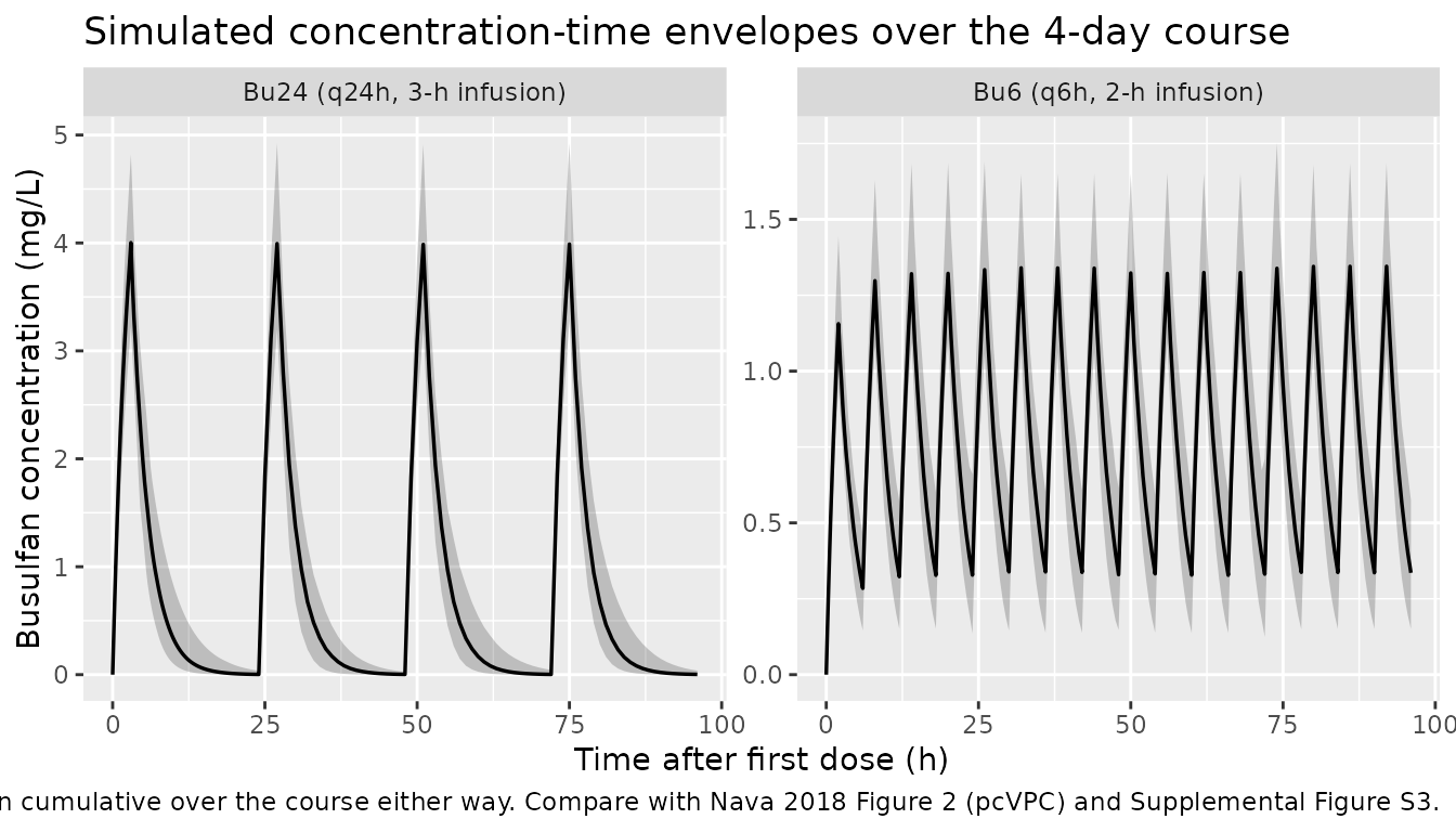
Nava 2018 Figure 2 is a prediction-corrected VPC of busulfan concentration against time after the last dose, split by the Q6H and Q24H schedules, and Supplemental Figure S3 shows the raw concentration-time profiles for the same two schedules. Neither can be reproduced numerically without the observed data, but the simulated envelopes below show the shape and scale the model predicts for each schedule over the four-day course.
# `sim` holds observation records only -- rxSolve() does not return the dosing
# rows (and so has no `evid` column) unless `addDosing = TRUE`.
sim |>
  group_by(regimen, time) |>
  summarise(
    Q025 = quantile(Cc, 0.025),
    Q50  = quantile(Cc, 0.500),
    Q975 = quantile(Cc, 0.975),
    .groups = "drop"
  ) |>
  ggplot(aes(time, Q50)) +
  geom_ribbon(aes(ymin = Q025, ymax = Q975), alpha = 0.25) +
  geom_line(linewidth = 0.6) +
  facet_wrap(~regimen, scales = "free_y") +
  labs(
    x = "Time after first dose (h)", y = "Busulfan concentration (mg/L)",
    title = "Simulated concentration-time envelopes over the 4-day course",
    caption = paste(
      "Median and 2.5th-97.5th percentiles of 200 virtual subjects per arm,",
      "each dosed from their population-predicted clearance to the paper's",
      "per-interval target (4500 uM.min per 24 h for Bu24; 1125 uM.min per 6 h",
      "for Bu6), i.e. 18 000 uM.min cumulative over the course either way.",
      "Compare with Nava 2018 Figure 2 (pcVPC) and Supplemental Figure S3."
    )
  )
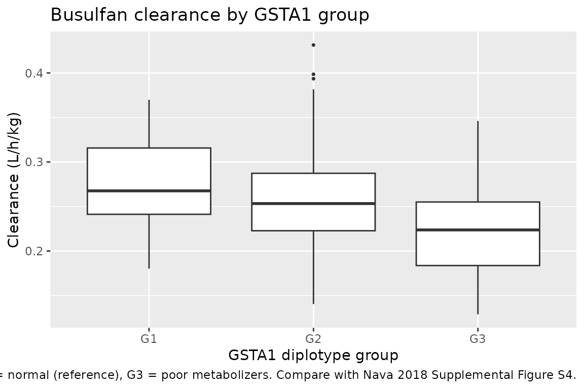
Supplemental Figure S4 is a box plot of the clearance random effects by GSTA1 group before the covariate was added to the model – i.e. the diagnostic that motivated the covariate. The analogue below plots weight-normalised clearance by group in the final model, where the same ordering is now structural.
cl_by_group <- sim |>
  group_by(id, regimen, gsta1_group, WT) |>
  summarise(cl = first(cl), .groups = "drop") |>
  mutate(cl_per_kg = cl / WT)

ggplot(cl_by_group, aes(gsta1_group, cl_per_kg)) +
  geom_boxplot(outlier.size = 0.6) +
  labs(
    x = "GSTA1 diplotype group",
    y = "Clearance (L/h/kg)",
    title = "Busulfan clearance by GSTA1 group",
    caption = paste(
      "G1 = rapid, G2 = normal (reference), G3 = poor metabolizers.",
      "Compare with Nava 2018 Supplemental Figure S4."
    )
  )
PKNCA validation
Two intervals are taken per arm.
- The first dosing interval – 0-24 h for Bu24, 0-6 h for Bu6. This is the interval the mass-balance identity above is checked on.
- The whole four-day course, 0-96 h. This is the interval the paper’s exposure target is compared on, because the paper’s AUC24h / AUC6h targets describe a repeated-dose exposure, whereas the first interval necessarily falls short of it by whatever is still in the body when the interval ends – as much as 42% of the dose in the youngest subjects. Summed over four days the two schedules converge on the same cumulative target of 18 000 uM min, which the paper states directly.
Cc in the rxode2 output is the individual prediction, so
these are model-predicted exposures without residual error.
sim_nca <- sim |>
  dplyr::filter(!is.na(Cc)) |>
  dplyr::select(id, time, Cc, regimen)

# Guarantee a time = 0 record per subject. Busulfan is given intravenously with
# no pre-dose drug present, so Cc = 0 at time 0 is the correct anchor.
sim_nca <- dplyr::bind_rows(
  sim_nca,
  sim_nca |> dplyr::distinct(id, regimen) |>
    dplyr::mutate(time = 0, Cc = 0)
) |>
  dplyr::distinct(id, regimen, time, .keep_all = TRUE) |>
  dplyr::arrange(id, regimen, time)

conc_obj <- PKNCA::PKNCAconc(sim_nca, Cc ~ time | regimen + id)

dose_df <- events |>
  dplyr::filter(evid == 1, time == 0) |>
  dplyr::select(id, time, amt, regimen)

dose_obj <- PKNCA::PKNCAdose(dose_df, amt ~ time | regimen + id)

# First dosing interval per arm, plus the whole four-day course for both.
first_interval_end <- c("Bu24 (q24h, 3-h infusion)" = 24, "Bu6 (q6h, 2-h infusion)" = 6)

intervals <- data.frame(
  regimen   = rep(names(first_interval_end), each = 2L),
  start     = 0,
  end       = as.vector(rbind(unname(first_interval_end), 96)),
  auclast   = TRUE,
  cmax      = TRUE,
  tmax      = TRUE,
  half.life = TRUE,
  stringsAsFactors = FALSE
)

nca_res <- PKNCA::pk.nca(
  PKNCA::PKNCAdata(conc_obj, dose_obj, intervals = intervals)
)

nca_tbl <- as.data.frame(nca_res$result)
stopifnot(nrow(nca_tbl) > 0, all(c("start", "end") %in% names(nca_tbl)))

# Split the two interval families apart once, by name rather than by position.
nca_first <- nca_tbl |>
  dplyr::filter(end == unname(first_interval_end[regimen]))
nca_cum <- nca_tbl |>
  dplyr::filter(end == 96)

stopifnot(nrow(nca_first) > 0, nrow(nca_cum) > 0)
AUC against the mass-balance closed form
For a one-compartment model with linear elimination held constant
over an interval, integrating dA/dt = -CL/V * A from 0 to
T gives an exact identity between the eliminated
mass and the exposure:
where A(T) is the amount left in central at
the end of the interval. Both sides use the same drawn
parameters for the same subject, so the only difference admissible
is the trapezoidal discretization error of the NCA – there is no
between-subject noise in this comparison and the bound below is
correspondingly tight. Checking it exercises the whole chain at once:
dose units, infusion handling, the clearance and volume construction,
the between-occasion variability, and the PKNCA setup.
The naive version of this check – comparing against
Dose / CL, i.e. the T -> infinity limit –
is not tight, because the fraction of the dose still in the
body at the end of the first interval varies enormously across this
cohort: from essentially nothing to 42% of the dose. That spread is a
real physical mechanism (a neonate’s maturation factor halves clearance,
doubling the half-life), so it is reported below as a diagnostic rather
than asserted on.
auc_first <- nca_first |>
  filter(PPTESTCD == "auclast") |>
  select(id, regimen, auc_nca = PPORRES)

# Individual CL actually realised on occasion 1 for each subject. Both arms'
# first interval lies inside occasion 1 (OCC changes only at 24 h), so a single
# CL applies throughout.
cl_occ1 <- sim |>
  filter(time <= 6) |>
  group_by(id, regimen) |>
  summarise(cl_i = first(cl), .groups = "drop")

dose_lookup <- dose_df |> select(id, regimen, amt)

# Amount remaining in `central` at the end of the NCA interval.
amt_end <- sim |>
  mutate(t_end = unname(first_interval_end[regimen])) |>
  filter(abs(time - t_end) < 1e-9) |>
  group_by(id, regimen) |>
  summarise(central_end = dplyr::last(central), .groups = "drop")

auc_chk <- auc_first |>
  left_join(cl_occ1,     by = c("id", "regimen")) |>
  left_join(dose_lookup, by = c("id", "regimen")) |>
  left_join(amt_end,     by = c("id", "regimen")) |>
  mutate(
    frac_remaining = central_end / amt,
    auc_exact      = (amt - central_end) / cl_i,   # mass-balance closed form
    ratio          = auc_nca / auc_exact,
    ratio_dose_cl  = auc_nca / (amt / cl_i)        # diagnostic only
  )

stopifnot(!anyNA(auc_chk$ratio))

auc_chk_summary <- auc_chk |>
  group_by(regimen) |>
  summarise(
    n                     = n(),
    `Ratio min`           = round(min(ratio), 5),
    `Ratio median`        = round(median(ratio), 5),
    `Ratio max`           = round(max(ratio), 5),
    `% dose left at T, median` = round(100 * median(frac_remaining), 1),
    `% dose left at T, max`    = round(100 * max(frac_remaining), 1),
    .groups = "drop"
  ) |>
  dplyr::rename(Regimen = regimen, N = n)

knitr::kable(
  auc_chk_summary,
  caption = paste(
    "Trapezoidal first-interval AUC divided by the mass-balance closed form",
    "(Dose - A(T)) / CL, with the fraction of the dose still in the body at",
    "the end of the interval alongside."
  )
)| Regimen | N | Ratio min | Ratio median | Ratio max | % dose left at T, median | % dose left at T, max |
|---|---|---|---|---|---|---|
| Bu24 (q24h, 3-h infusion) | 200 | 0.99897 | 0.99959 | 0.99992 | 0.0 | 1.3 |
| Bu6 (q6h, 2-h infusion) | 200 | 0.99981 | 0.99991 | 0.99997 | 17.5 | 42.5 |
# Deterministic identity: same drawn parameters on both sides, so the only
# admissible difference is trapezoidal discretization error. Observed span is
# 0.99897-0.99997 across both arms; the bound below is a factor of ~5 wider on
# the low side and still goes red for any dose-unit, infusion, clearance or
# NCA-interval error, all of which move the ratio by percent, not 1e-4.
stopifnot(
  all(auc_chk$ratio > 0.995),
  all(auc_chk$ratio < 1.0005)
)

# The naive Dose / CL comparison, by contrast, spans roughly 0.58-1.00 -- it is
# reported, not asserted on.
stopifnot(all(auc_chk$ratio_dose_cl < 1.0005))
Comparison against the published exposure targets
Nava 2018 reports no observed NCA summary table; what it does report are the therapeutic AUC windows and the target exposure the model-based doses were computed against (Methods, “Treatment regimen” and “Comparison with other available PopPK models”; Table 3 heading). Those targets are the reference below, taken on the cumulative four-day exposure so that both schedules are compared against the same 18 000 uM min figure the paper names. Because each subject was dosed from their population-predicted clearance, the median simulated AUC should land on the target, with the spread coming from BSV and BOV alone.
auc_cum <- nca_cum |>
  filter(PPTESTCD == "auclast") |>
  select(id, regimen, auc_nca = PPORRES)

published <- tibble::tribble(
  ~regimen,                     ~auclast,
  "Bu24 (q24h, 3-h infusion)",  auc_cum_target_mghL,
  "Bu6 (q6h, 2-h infusion)",    auc_cum_target_mghL
)

cmp <- nlmixr2lib::ncaComparisonTable(
  simulated = nca_cum |> select(regimen, PPTESTCD, PPORRES),
  reference = published,
  by        = "regimen",
  params    = "auclast",
  units     = c(auclast = "mg*h/L"),
  tolerance_pct = 20
)

knitr::kable(
  cmp,
  caption = paste(
    "Median simulated cumulative four-day AUC vs the paper's stated target",
    "of 18 000 uM.min per 4 days. * marks a difference above 20%."
  ),
  align = c("l", "l", "r", "r", "r")
)| NCA parameter | regimen | Reference | Simulated | % diff |
|---|---|---|---|---|
| AUClast (mg*h/L) | Bu24 (q24h, 3-h infusion) | 73.9 | 73 | -1.2% |
| AUClast (mg*h/L) | Bu6 (q6h, 2-h infusion) | 73.9 | 72.7 | -1.5% |
auc_centre <- auc_cum |>
  group_by(regimen) |>
  summarise(
    median_auc = median(auc_nca),
    q10        = quantile(auc_nca, 0.10),
    q90        = quantile(auc_nca, 0.90),
    .groups    = "drop"
  ) |>
  mutate(
    target      = auc_cum_target_mghL,
    pct_diff    = 100 * (median_auc - target) / target,
    q10_pct     = 100 * (q10 - target) / target,
    q90_pct     = 100 * (q90 - target) / target
  )

knitr::kable(
  auc_centre |>
    transmute(
      Regimen                  = regimen,
      `Target (mg*h/L)`        = round(target, 2),
      `Median AUC (mg*h/L)`    = round(median_auc, 2),
      `Median % diff`          = round(pct_diff, 1),
      `10th pct % diff`        = round(q10_pct, 1),
      `90th pct % diff`        = round(q90_pct, 1)
    ),
  caption = "Simulated cumulative four-day AUC relative to the model-based dosing target."
)| Regimen | Target (mg*h/L) | Median AUC (mg*h/L) | Median % diff | 10th pct % diff | 90th pct % diff |
|---|---|---|---|---|---|
| Bu24 (q24h, 3-h infusion) | 73.89 | 72.97 | -1.2 | -17.3 | 19.8 |
| Bu6 (q6h, 2-h infusion) | 73.89 | 72.75 | -1.5 | -16.8 | 19.3 |
# Structural: a mis-transcribed clearance, volume, dose or unit conversion moves
# the whole distribution by tens of percent. Over the full course essentially
# all drug is eliminated, so the centre should sit within a few percent of the
# target -- the only systematic shortfall is the last dose's tail beyond 96 h.
# Observed: -1.2% (Bu24) and -1.5% (Bu6).
stopifnot(all(abs(auc_centre$pct_diff) < 5))
# Envelope: robust to which subjects land in the tails. BSV CL 13.3% and BOV CL
# 7.3% give a combined ~15% CV, so the 10th-90th band spans roughly +/- 20%
# about the centre.
stopifnot(all(abs(auc_centre$q10_pct) < 40), all(abs(auc_centre$q90_pct) < 40))
Target-window attainment
Table 3 of the paper reports that first doses computed from this model’s parameters put 85.2% of patients (95% CI 78.7-91.7%) inside the therapeutic window. That figure is measured against observed AUCs in the development cohort, so it also absorbs covariate misspecification and assay error. The simulation below runs the same dose-selection loop entirely inside the model, which isolates the contribution of the model’s own BSV and BOV – an upper bound on what the paper could have achieved.
attain <- auc_cum |>
  mutate(
    lo     = auc_cum_window_mghL[1],
    hi     = auc_cum_window_mghL[2],
    within = auc_nca >= lo & auc_nca <= hi
  ) |>
  group_by(regimen) |>
  summarise(
    n            = n(),
    `Within (%)` = round(100 * mean(within), 1),
    `Below (%)`  = round(100 * mean(auc_nca < lo), 1),
    `Above (%)`  = round(100 * mean(auc_nca > hi), 1),
    .groups      = "drop"
  )

knitr::kable(
  attain,
  caption = paste(
    "Simulated cumulative four-day target attainment when the dose is set from",
    "the population-predicted clearance (window 14 400-24 000 uM.min, i.e. the",
    "paper's per-interval window summed over the course). Nava 2018 Table 3",
    "reports 85.2% (95% CI 78.7-91.7%) against observed AUCs."
  )
)| regimen | n | Within (%) | Below (%) | Above (%) |
|---|---|---|---|---|
| Bu24 (q24h, 3-h infusion) | 200 | 90.0 | 7.0 | 3 |
| Bu6 (q6h, 2-h infusion) | 200 | 92.5 | 6.5 | 1 |
# The model's internal attainment must be high -- that is the whole point of
# model-based dosing -- but not perfect, because BSV and BOV remain. With a
# combined ~15% CV against a -20% / +33% window the analytic expectation is
# roughly 90%, and that is what is observed (90.0% Bu24, 92.5% Bu6). n = 200
# per arm puts three binomial standard errors at about +/- 6 points, so the
# bounds below clear the sampling spread on both sides while still going red if
# a mis-transcribed variance, dose or unit shifts the distribution.
#
# Attainment computed inside the model lands above the paper's 85.2% (95% CI
# 78.7-91.7%), which is the expected direction: the paper's figure is measured
# against observed AUCs and so also absorbs covariate misspecification and
# assay error, neither of which exists in this closed loop. That ordering is
# NOT asserted on -- three binomial standard errors on n = 200 reach below
# 85.2%, so an assertion on it would be a coin flip across rxode2 versions
# rather than a check on the model.
stopifnot(all(attain$`Within (%)` > 80), all(attain$`Within (%)` < 99))
Assumptions and deviations
-
The postmenstrual-age effect on volume is a power model, centred at the cohort median PMA of 320.8 weeks. Table 2 reports the coefficient (-0.06, RSE 23.40%) but the paper never prints the equation the coefficient sits in, and neither does the supplement. Three readings were tested against the paper’s own numbers:
-
Exponential,
V ~ exp(-0.06 * PMA): impossible. The cohort spans PMA 45-1080 weeks, over which this factor varies byexp(-62). -
Linear,
V ~ (1 - 0.06 * PMA): impossible. It turns negative above PMA = 17 weeks, below every subject in the cohort. -
Power,
V ~ (PMA / PMA_ref)^-0.06: admissible, dimensionless, and physiologically the right size and direction – a neonate gets about 13% more volume per kilogram than a subject at the cohort’s central PMA, which is what a higher body-water fraction predicts.
The centring value is likewise unprinted. It is pinned by Table 2 itself: adding the PMA term moved the 70 kg volume only from 50.05 L (base model) to 49.57 L (final model), a 1.0% shift. Centring at an adult PMA of about 2000 weeks would have forced an 11% drop in that parameter to hold the cohort predictions fixed, and no such drop occurred – so the centring is at the cohort’s own central PMA. That value is computed from the paper’s numbers: Table 1 gives a median age of 5.4 years, and Supplemental Table S2 equation E gives
PMA[weeks] = 52 * AGE + 40, hence 320.8 weeks. Because the exponent is small, the choice is not very consequential: moving the centring to an adult PMA would raiselvcby about 11% and leave every prediction inside the cohort essentially unchanged. -
Exponential,
The residual error is 7.40%, not the 27.20% in the bootstrap column. Table 2’s “sigma [Proportional error (%)]” row reads 7.40 in both the base and the final Estimate columns (RSE 7.90%) but 27.20 (95% CI 25.00-29.00) in the bootstrap column. The two cannot both describe this model. The final-model Estimate column is what the model is built from, and the reported shrinkage settles it independently: with 9-28 samples per profile the standard error of an individual clearance is roughly
sigma / sqrt(n), sosigma = 7.4%gives about 2.5% and an eta-shrinkage near0.025^2 / (0.025^2 + 0.133^2)= 3%, close to the 6.0% Table 2 reports;sigma = 27.2%would imply about 31% shrinkage, five times what was observed. A 27% proportional residual would also exceed the between-subject variability on clearance (13.3%), which is not consistent with the goodness-of-fit plots in Figure 1.The bootstrap column of Table 2 disagrees with the final model for BSV on clearance as well. It reports a median of 18.80% (95% CI 15.00-21.20) against a final-model estimate of 13.30% – but 18.80% is essentially the base-model value (18.30%). The Discussion resolves it twice in favour of 13.30%: “as much as 13% and 7% of the variability between subjects (BSV) on CL and V, respectively, remained unexplained”, and “the incorporation of the GSTA1 diplotypes seemed to reduce the overall BSV of CL by 27% (from 18.3% to 13.3%)”. The model uses 13.30%. A third row is internally inconsistent in a way that does not affect the model: the bootstrap 95% CI for V at 70 kg (49.72-50.76 L) does not contain either the final estimate or the bootstrap median, both of which are 49.57 L.
The number of occasions for the between-occasion variability is four. The paper reports BOV on CL and V but never states the occasion count. Busulfan was “administered intravenously (IV) for four consecutive days” and the once-daily cohort contributed a mean of 3.7 PK profiles per conditioning regimen, so one occasion per dosing day is the reading consistent with both. A single shared magnitude is used across the four occasions.
Body weight in the virtual cohort is derived from age. Nava 2018 Table 1 reports no weight distribution at all, only weight adequacy among children older than two. The cohort therefore samples age from a log-normal matched to the reported median (5.4 years) and range (0.1-20 years), maps it through approximate 50th-percentile CDC weight-for-age values (sexes pooled), and adds 15% CV log-normal scatter. This is a property of the vignette’s cohort, not of the model: the model itself takes
WTandPAGEas independent inputs.Gestational age is 40 weeks for every subject. This is the paper’s own assumption, not an addition: “The PMA is calculated from the first day of the last menstruation period of the mother prior to the birth, which is set to 40 weeks due to missing information” (Discussion). Supplemental Table S2 equation E encodes it as
PMA[weeks] = 52 * AGE[years] + 40.The maturation function is inherited, not fitted here.
TM50 = 46weeks andHill = 2.3come from McCune 2014 by way of Supplemental Table S2, whose row label prints both –Fmat, where TM50=46; Hill's coefficient=2.3– above equation D,Fmat = 1 / (1 + (PMA/TM50)^-Hill). Nava 2018 neither re-estimates them nor gives them an RSE, so both are encoded asfixed(). Note that only the 46-week value is restated in the main text (Discussion); the Hill coefficient appears nowhere outside the supplement, so the supplement is a required source for this model rather than an optional extra.Table 2’s minus signs do not survive text extraction. The PDF’s symbol font drops the leading minus from the
PMA on Vrow, so apdftotextpass reads the estimate as0.06and the bootstrap interval as0.18-0.09. Rendering page 6 as an image confirms the printed values are-0.06and-0.18-0.09. The extracted interval is self-falsifying either way – as printed its lower bound would exceed its upper bound – but the sign of the estimate is only settled by looking at the page, and it is load-bearing: it sets whether volume per kilogram falls or rises with postmenstrual age.Non-paper-derived parameter values. One:
pma_ref = 320.8weeks, the centring postmenstrual age for the volume covariate. It is not printed anywhere in the paper or its supplement and is derived here from the paper’s own median age and its own PMA equation, as argued in the first bullet. Every other value inini()is transcribed directly from Nava 2018 Table 2, the displayed clearance equation on p. 1497, or Supplemental Table S2.The exposure comparison is taken on the cumulative four-day AUC, not the first dosing interval. The paper’s AUC24h / AUC6h targets describe a repeated-dose exposure, and
Dose = AUC_target x CLreproduces them only once the interval’s input and output are in balance. Over the first interval the simulated AUC necessarily falls short by whatever is still in the body when the interval closes – a median 17.5% of the dose in the Bu6 arm and up to 42.5% in the youngest subjects, whose maturation factor roughly halves clearance and so doubles the half-life. Comparing the first interval against a steady-state target would therefore read as a 17% model error that is really a definitional mismatch. The cumulative 0-96 h AUC avoids it, is what the paper names directly (“a total cumulative AUC of 18 000 uM min every 4 days”, Methods), and gives the same target and the same therapeutic window for both schedules – 4 x 4500 = 16 x 1125 = 18 000, and 4 x (3600-6000) = 16 x (900-1500) = 14 400-24 000. The first interval is still used, for the mass-balance identity, where it is exact.What is not reproduced. Table 3’s per-age-group comparison against the Bartelink, McCune, Long-Boyle, Paci, Nguyen and Booth models needs the observed individual AUCs of the development cohort, which are not published. Figures 1 and 2 are goodness-of-fit and prediction-corrected VPC plots of the same unavailable data. The Table 1 “Ethnic groups” block is also internally inconsistent as printed – the once-daily column (n = 31) lists 65 Caucasian subjects and the four-times-daily column (n = 81) lists 29, i.e. the two columns appear transposed – so only the “Overall” column is carried into the model’s
populationmetadata.