Caspofungin (Abdul-Aziz 2025)
Source:vignettes/articles/AbdulAziz_2025_caspofungin.Rmd
AbdulAziz_2025_caspofungin.RmdModel and source
- Citation: Abdul-Aziz MH, Diehl A, Liu X, Cheng V, Corley A, Gilder E, Levkovich B, McGuinness S, Ordonez J, Parke R, Pellegrino V, Wallis SC, Fraser JF, Shekar K, Roberts JA. Population pharmacokinetics of caspofungin in critically ill patients receiving extracorporeal membrane oxygenation-an ASAP ECMO study. Antimicrob Agents Chemother. 2025;69(2):e01435-24. doi:10.1128/aac.01435-24. PMC11823646. Published online 18 December 2024.
- Description: One-compartment population PK model with first-order elimination for intravenous caspofungin in critically ill adults receiving extracorporeal membrane oxygenation (ECMO), from the ASAP ECMO study program. Central volume scales with Janmahasatian fat-free mass (reported by the source as lean body weight) through an estimated power exponent of 1.24 standardised to the cohort median of 58.9 kg; clearance carries no covariate. Every patient in the cohort was cannulated onto ECMO, so ECMO support is a property of the population rather than a covariate – ECMO duration, mode and flow rate were all screened and none was retained, which is the paper’s central negative finding. Estimated by SAEM in Monolix 2021R2 with an additive residual error. Abdul-Aziz 2025, n = 8 patients, 64 plasma samples over a single dosing interval.
- Article: https://doi.org/10.1128/aac.01435-24
- Open-access full text: https://www.ncbi.nlm.nih.gov/pmc/articles/PMC11823646/
This is a one-compartment model with first-order elimination for intravenous caspofungin in critically ill adults on extracorporeal membrane oxygenation (ECMO), from the ASAP ECMO study program. It is a deliberately small model: two structural parameters, one covariate, and an additive residual error. That makes it unusually amenable to exact verification, and the sections below take advantage of that – every structural claim is checked against a closed form rather than against a picture.
Population
Eight critically ill adults contributed 64 plasma concentration-time points, sampled over a single dosing interval once the patient had been stabilised on ECMO (Abdul-Aziz 2025 Results, “Study population characteristics”). The cohort median age was 36.5 years (range 20.0-62.0), actual body weight 84.0 kg (range 55.0-130.0), and lean body weight 58.9 kg (range 37.3-81); 5 of 8 (62.5%) were male (Table 1). All patients were hypoalbuminaemic (albumin 17-33 g/L) and renal function spanned impairment to markedly augmented clearance (Cockcroft-Gault creatinine clearance median 57.0 mL/min, range 31.0-260.0).
Every patient was cannulated onto ECMO – veno-venous in 6 (75.0%) and veno-arterial in 2 (25.0%) – and 5 of 8 (62.5%) received concomitant renal replacement therapy during sampling (4 CVVHD, 1 SLED). ECMO support is therefore a property of this population rather than a covariate in the model: the indicator is constant at 1 and cannot be estimated. The ECMO variables that do vary within the cohort (duration, mode, flow rate) were all screened and none was retained, which is the paper’s headline finding – “the use of ECMO had negligible impact on the pharmacokinetics of caspofungin in critically ill patients” (Discussion).
All patients received a 70 mg loading dose on day 1 as a 1 h infusion, followed by a daily maintenance dose of 50 mg (6 patients) or 70 mg (2 patients). The virtual cohort below reproduces that 6:2 split.
The same information is available programmatically via the model’s
population metadata
(readModelDb("AbdulAziz_2025_caspofungin")()$population).
Source trace
The per-parameter origin is recorded as an in-file comment next to
each ini() entry in
inst/modeldb/specificDrugs/AbdulAziz_2025_caspofungin.R.
The table below collects them in one place for review.
| Equation / parameter | Value | Source location |
|---|---|---|
lcl (CL) |
0.55 L/h | Table 2, “CL (L/h)” = 0.55 (%RSE 11.9); bootstrap median 0.55 (95% CI 0.42-0.68); restated in the Abstract |
lvc (V at FFM = 58.9 kg) |
8.13 L | Table 2, “V (L)” = 8.13 (%RSE 7.15); bootstrap median 8.27 (95% CI 7.07-10.8); restated in the Abstract |
e_ffm_vc |
1.24 | Table 2, “LBW effect on V” = 1.24 (%RSE 23.3); bootstrap median 1.24 (95% CI 0.08-1.91) |
etalcl (BSV on CL) |
0.062996 = log(1 + 0.255^2) | Table 2, BSV “CL (%)” = 25.5 (%RSE 34.3) |
etalvc (BSV on V) |
0.0054758 = log(1 + 0.0741^2) | Table 2, BSV “V (%)” = 7.41 (%RSE 101) |
addSd |
1.20 mg/L | Table 2, Residual error “Additive (mg/L)” = 1.20 (%RSE 10.0) |
vc <- exp(lvc + etalvc) * (FFM / 58.9)^e_ffm_vc |
n/a | Displayed equation in Results, “Covariate screening and model
development”: V = Vpop * (LBW / 58.9)^1.24. The 58.9 kg
divisor is the cohort median lean body weight (Table 1), per the Methods
statement that continuous covariates were centred on their medians |
cl <- exp(lcl + etalcl) |
n/a | Methods, “Structural model development”: BSV “described using an
exponential model” theta_j = theta_p * exp(eta_j). No
covariate retained on clearance (serum albumin was tested and
rejected) |
d/dt(central) <- -kel * central |
n/a | Results, “Population pharmacokinetic model building”: “best described by a one-compartment model with first-order elimination”; a two-compartment model did not reduce BICc |
Cc ~ add(addSd) |
n/a | Results: “Residual unexplained variability was described by an additive error model” |
| Reference FFM = 58.9 kg | 58.9 kg | Table 1, “Lean body weight (in kg)” median 58.9 (range 37.3-81); also the divisor printed in the covariate equation |
The LBW label used throughout the paper is registered
here as the canonical covariate FFM. The register
discriminates fat-free mass from lean body mass by the estimating
formula, not by the paper’s label, and Abdul-Aziz 2025 cites
Janmahasatian et al. – the fat-free-mass equation. The paper itself
makes the identification explicit: “Although the Janmahasatian et
al. equation was developed to estimate fat-free mass, the estimate is
considered to be a representation of lean body weight and is commonly
used interchangeably” (Discussion). This follows the identical
LBW -> FFM precedent in
Rolsma_2025_cefepime.R.
Structural verification against closed forms
A one-compartment model with first-order elimination has exact analytic identities, so these checks compare the packaged model against arithmetic derived from the paper’s printed numbers (0.55 L/h, 8.13 L, exponent 1.24, 58.9 kg) rather than against a digitised figure. They are deterministic – typical values with the random effects zeroed – so the tolerances are tight on purpose: the residual difference is pure numerical error, not cohort sampling.
mod <- readModelDb("AbdulAziz_2025_caspofungin")
mod_typ <- rxode2::zeroRe(mod)

# The paper's printed values, transcribed once and reused below.
pub_cl  <- 0.55  # L/h,  Table 2
pub_v   <- 8.13  # L,    Table 2 (at FFM = 58.9 kg)
pub_exp <- 1.24  # -,    Table 2 "LBW effect on V"
pub_ref <- 58.9  # kg,   Table 1 median lean body weight

# Build a typical-value event table: 70 mg loading dose then `md` mg q24h,
# each as a 1 h intravenous infusion into the central compartment.
make_events <- function(md, ffm, ndays, by = 0.02, id = 1L,
                        obs_end = 24 * ndays) {
  amts <- c(70, rep(md, ndays - 1L))
  dose <- data.frame(
    id = id, time = seq(0, by = 24, length.out = ndays),
    amt = amts, rate = amts, # rate = amt / 1 h infusion
    evid = 1L, cmt = "central", FFM = ffm
  )
  obs <- data.frame(
    id = id, time = seq(0, obs_end, by = by),
    amt = NA_real_, rate = NA_real_,
    evid = 0L, cmt = "central", FFM = ffm
  )
  rbind(dose, obs)
}
Fat-free-mass power scaling
The volume must equal 8.13 * (FFM / 58.9)^1.24 at every
fat-free mass, and must equal exactly 8.13 L at the reference. Checked
across the full observed range of the cohort (37.3-81 kg) plus the four
values the paper simulated (40, 50, 60, 80 kg).
ffm_grid <- c(37.3, 40, 50, 58.9, 60, 80, 81)
ffm_chk <- vapply(ffm_grid, function(f) {
  s <- rxode2::rxSolve(mod_typ, make_events(50, f, ndays = 1L, by = 12),
                       returnType = "data.frame")
  unique(s$vc)[1]
}, numeric(1))
#> ℹ omega/sigma items treated as zero: 'etalcl', 'etalvc'
#> ℹ omega/sigma items treated as zero: 'etalcl', 'etalvc'
#> ℹ omega/sigma items treated as zero: 'etalcl', 'etalvc'
#> ℹ omega/sigma items treated as zero: 'etalcl', 'etalvc'
#> ℹ omega/sigma items treated as zero: 'etalcl', 'etalvc'
#> ℹ omega/sigma items treated as zero: 'etalcl', 'etalvc'
#> ℹ omega/sigma items treated as zero: 'etalcl', 'etalvc'

ffm_tab <- data.frame(
  FFM = ffm_grid,
  model = ffm_chk,
  closed_form = pub_v * (ffm_grid / pub_ref)^pub_exp
)
ffm_tab$rel_diff <- abs(ffm_tab$model - ffm_tab$closed_form) / ffm_tab$closed_form

ffm_tab |>
  dplyr::rename(
    "FFM (kg)"                    = FFM,
    "Model Vc (L)"                = model,
    "8.13 * (FFM/58.9)^1.24 (L)"  = closed_form,
    "Relative difference"         = rel_diff
  ) |>
  knitr::kable(digits = c(1, 4, 4, 12),
caption = "Central volume vs the paper's displayed covariate equation.")| FFM (kg) | Model Vc (L) | 8.13 * (FFM/58.9)^1.24 (L) | Relative difference |
|---|---|---|---|
| 37.3 | 4.6139 | 4.6139 | 0 |
| 40.0 | 5.0316 | 5.0316 | 0 |
| 50.0 | 6.6355 | 6.6355 | 0 |
| 58.9 | 8.1300 | 8.1300 | 0 |
| 60.0 | 8.3187 | 8.3187 | 0 |
| 80.0 | 11.8845 | 11.8845 | 0 |
| 81.0 | 12.0689 | 12.0689 | 0 |
Terminal half-life
For a one-compartment model, t1/2 = log(2) * V / CL.
Recovered here by regressing log(Cc) on time over a window
well clear of the last infusion, so the estimate comes from the
solved concentrations rather than from the model’s own
kel output column (a gate built from a model variable
cannot go red).
s_hl <- rxode2::rxSolve(
  mod_typ,
  # Dose for 5 days, then observe well past the last dose so a terminal
  # window is actually available to regress over.
  make_events(50, pub_ref, ndays = 5L, by = 0.25, obs_end = 220),
  returnType = "data.frame"
)
#> ℹ omega/sigma items treated as zero: 'etalcl', 'etalvc'
# Last infusion ends at 97 h; regress 130-200 h (>3 half-lives clear of it).
# Keep Cc >= 1e-6 * Cmax: below that the ODE integrator has no relative accuracy left.
w_hl <- s_hl[!is.na(s_hl$Cc) & s_hl$time >= 130 & s_hl$time <= 200 &
               s_hl$Cc >= 1e-6 * max(s_hl$Cc, na.rm = TRUE), ]
stopifnot(nrow(w_hl) > 50) # a regression on zero rows must not pass silently
kel_fit <- -unname(coef(lm(log(Cc) ~ time, data = w_hl))[2])

hl_model <- log(2) / kel_fit
hl_closed <- log(2) * pub_v / pub_cl
c(measured_h = hl_model, closed_form_h = hl_closed,
  rel_diff = abs(hl_model - hl_closed) / hl_closed)
#>    measured_h closed_form_h      rel_diff
#>  1.024598e+01  1.024598e+01  3.763888e-13

stopifnot(abs(hl_model - hl_closed) / hl_closed < 1e-6)
Mass-balance AUC identity
For any linear model with elimination only from the central compartment,
AUC(0, T) == (amount infused by T - amount remaining at T) / CLholds exactly at any T, in or out of steady state. That makes it the strongest available gate for a paper whose sampling covered only a single dosing interval: it needs no steady-state assumption and no extrapolation. A mis-transcribed clearance, dose, infusion duration or ODE sign breaks it immediately.
s_mb <- rxode2::rxSolve(mod_typ, make_events(50, pub_ref, ndays = 6L, by = 0.02),
                        returnType = "data.frame")
#> ℹ omega/sigma items treated as zero: 'etalcl', 'etalvc'
o_mb <- s_mb[!is.na(s_mb$Cc), ]

trap <- function(t, y) sum(diff(t) * (utils::head(y, -1) + utils::tail(y, -1)) / 2)

# Amount actually infused by time T, valid mid-infusion as well as after it.
infused_by <- function(T, dose_times, dose_amts, dur = 1) {
  sum(dose_amts * pmin(pmax(T - dose_times, 0), dur) / dur)
}
dose_times <- seq(0, by = 24, length.out = 6L)
dose_amts <- c(70, rep(50, 5L))

mb <- do.call(rbind, lapply(c(0.5, 6, 12, 24, 36, 48, 100, 144), function(T) {
  w <- o_mb[o_mb$time <= T, ]
  lhs <- trap(w$time, w$Cc)
  rhs <- (infused_by(T, dose_times, dose_amts) - w$central[nrow(w)]) / pub_cl
  data.frame(T = T, auc_trapezoid = lhs, auc_mass_balance = rhs,
             rel_diff = abs(lhs - rhs) / rhs)
}))

mb |>
  dplyr::rename(
    "T (h)"                      = T,
    "AUC(0,T) trapezoid (mg.h/L)" = auc_trapezoid,
    "(infused - remaining)/CL"    = auc_mass_balance,
    "Relative difference"         = rel_diff
  ) |>
  knitr::kable(digits = c(1, 4, 4, 10),
caption = "Mass-balance AUC identity, exact at every T including mid-infusion (T = 0.5 h).")| T (h) | AUC(0,T) trapezoid (mg.h/L) | (infused - remaining)/CL | Relative difference |
|---|---|---|---|
| 0.5 | 1.0642 | 1.0642 | 8.9759e-06 |
| 6.0 | 39.5269 | 39.5269 | 3.2570e-07 |
| 12.0 | 68.8012 | 68.8012 | 1.2220e-07 |
| 24.0 | 101.3082 | 101.3082 | 3.4000e-08 |
| 36.0 | 164.8868 | 164.8867 | 4.5820e-07 |
| 48.0 | 194.5160 | 194.5159 | 4.1160e-07 |
| 100.0 | 401.5120 | 401.5117 | 9.5520e-07 |
| 144.0 | 558.7165 | 558.7160 | 8.9780e-07 |
Steady-state AUC over a dosing interval
At steady state AUC(0, tau) == Dose / CL, so the typical
patient’s day-to-day exposure on 50 mg and 70 mg maintenance dosing is
pinned by clearance alone.
ss_chk <- do.call(rbind, lapply(c(50, 70), function(md) {
  s <- rxode2::rxSolve(mod_typ, make_events(md, pub_ref, ndays = 12L, by = 0.02),
                       returnType = "data.frame")
  o <- s[!is.na(s$Cc), ]
  w <- o[o$time >= 264 & o$time <= 288, ] # final interval, ~26 half-lives in
  data.frame(dose_mg = md, auc_solved = trap(w$time, w$Cc),
             auc_closed = md / pub_cl)
}))
#> ℹ omega/sigma items treated as zero: 'etalcl', 'etalvc'
#> ℹ omega/sigma items treated as zero: 'etalcl', 'etalvc'
ss_chk$rel_diff <- abs(ss_chk$auc_solved - ss_chk$auc_closed) / ss_chk$auc_closed

ss_chk |>
  dplyr::rename(
    "Maintenance dose (mg)"            = dose_mg,
    "AUC(0,tau) solved (mg.h/L)"       = auc_solved,
    "Dose/CL (mg.h/L)"                 = auc_closed,
    "Relative difference"              = rel_diff
  ) |>
  knitr::kable(digits = c(0, 4, 4, 10),
caption = "Steady-state AUC over the 24 h dosing interval vs Dose/CL.")| Maintenance dose (mg) | AUC(0,tau) solved (mg.h/L) | Dose/CL (mg.h/L) | Relative difference |
|---|---|---|---|
| 50 | 90.9092 | 90.9091 | 1.2039e-06 |
| 70 | 127.2729 | 127.2727 | 1.1979e-06 |
Virtual cohort
Original observed data are not publicly available. The cohort below reproduces the study’s actual regimen mix: a 70 mg loading dose for everyone, then 50 mg q24h in 75% of subjects and 70 mg q24h in 25%, matching the paper’s 6:2 split. Fat-free mass is drawn log-normally, centred on the cohort median of 58.9 kg and truncated to the observed range of 37.3-81 kg (Table 1).
Cohort size is 200 subjects, the per-arm cap for these vignettes. The paper simulated 500 for its VPC and 1,000 for its dosing simulations; 200 is ample to reproduce the published threshold claims and keeps the render fast.
# `set.seed()` seeds R's RNG (used for the covariate draw). It does NOT seed
# rxode2's simulation RNG, and rxode2's streams are partitioned PER SOLVER
# THREAD -- so the eta draws below are reproducible on this machine and differ
# on a machine with a different thread count. Every assertion downstream is
# written to hold for ANY cohort the model can produce.
set.seed(11823646)
rxode2::rxSetSeed(11823646)

n_sub <- 200L
ffm_draw <- pmin(pmax(pub_ref * exp(rnorm(n_sub, 0, 0.28)), 37.3), 81)
md_draw <- ifelse(seq_len(n_sub) <= round(n_sub * 6 / 8), 50, 70)

subj <- tibble::tibble(
  id = seq_len(n_sub),
  FFM = ffm_draw,
  md = md_draw,
  regimen = paste0("LD 70 mg, MD ", md_draw, " mg q24h"),
  cohort = "As studied (70 mg LD; 50 mg in 75%, 70 mg in 25%)"
)

# The paper's sampling schedule (Methods, "Study procedures"), applied to the
# day-1 and day-2 intervals, plus a fine grid over day 2 for the NCA.
samp <- c(0, 0.25, 0.5, 0.75, 1, 1.5, 2, 3, 6, 8, 12, 24)
obs_times <- sort(unique(c(samp, 24 + samp, seq(24, 48, by = 0.25))))

events <- dplyr::bind_rows(
  subj |>
    tidyr::expand_grid(time = c(0, 24)) |>
    dplyr::mutate(
      amt = ifelse(time == 0, 70, md),
      rate = amt,
      evid = 1L,
      cmt = "central"
    ),
  subj |>
    tidyr::expand_grid(time = obs_times) |>
    dplyr::mutate(amt = NA_real_, rate = NA_real_, evid = 0L, cmt = "central")
) |>
  dplyr::arrange(id, time, dplyr::desc(evid)) |>
  dplyr::select(id, time, amt, rate, evid, cmt, FFM, md, regimen, cohort)

stopifnot(!anyDuplicated(unique(events[, c("id", "time", "evid")])))
c(subjects = n_sub, md50 = sum(md_draw == 50), md70 = sum(md_draw == 70),
  ffm_median = median(ffm_draw))
#>   subjects       md50       md70 ffm_median
#>  200.00000  150.00000   50.00000   57.86014
Simulation
sim <- rxode2::rxSolve(
  mod, events = events,
  keep = c("regimen", "cohort", "md", "FFM")
) |>
  as.data.frame()

# `Cc` is the individual prediction (IPRED). The additive residual SD of
# 1.20 mg/L is large relative to late-interval troughs, so residual-perturbed
# observations can go negative; the exposure checks below use `Cc`.
stopifnot(all(sim$Cc[!is.na(sim$Cc)] >= 0))
Replicating Figure 2 (visual predictive check)
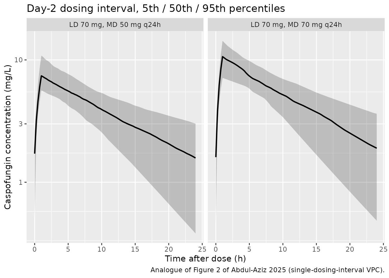
Figure 2 of Abdul-Aziz 2025 is a VPC over the single sampled dosing interval. The panels below show the 5th, 50th and 95th percentiles of the model’s predictions over the day-2 interval, re-referenced to time after dose, split by the maintenance dose actually received.
sim |>
  dplyr::filter(!is.na(Cc), time >= 24, time <= 48) |>
  dplyr::mutate(tad = time - 24) |>
  dplyr::group_by(regimen, tad) |>
  dplyr::summarise(
    Q05 = quantile(Cc, 0.05), Q50 = quantile(Cc, 0.50),
    Q95 = quantile(Cc, 0.95), .groups = "drop"
  ) |>
  ggplot(aes(tad, Q50)) +
  geom_ribbon(aes(ymin = Q05, ymax = Q95), alpha = 0.25) +
  geom_line(linewidth = 0.8) +
  facet_wrap(~regimen) +
  scale_y_log10() +
  labs(
    x = "Time after dose (h)", y = "Caspofungin concentration (mg/L)",
    title = "Day-2 dosing interval, 5th / 50th / 95th percentiles",
    caption = "Analogue of Figure 2 of Abdul-Aziz 2025 (single-dosing-interval VPC)."
  )
PKNCA validation
Non-compartmental analysis over the day-2 dosing interval (24-48 h), stratified by the maintenance dose received.
# Use only `!is.na(Cc)` -- adding `time > 0` or `Cc > 0` would drop the
# interval-anchoring records PKNCA needs.
sim_nca <- sim |>
  dplyr::filter(!is.na(Cc)) |>
  dplyr::select(id, time, Cc, regimen, cohort)

conc_obj <- PKNCA::PKNCAconc(
  as.data.frame(sim_nca), Cc ~ time | regimen + id,
  concu = "mg/L", timeu = "h"
)

dose_df <- events |>
  dplyr::filter(evid == 1, time == 24) |>
  dplyr::select(id, time, amt, regimen)

dose_obj <- PKNCA::PKNCAdose(as.data.frame(dose_df), amt ~ time | regimen + id,
                             doseu = "mg")

intervals <- data.frame(
  start = 24, end = 48,
  cmax = TRUE, tmax = TRUE, cmin = TRUE,
  auclast = TRUE, cav = TRUE, half.life = TRUE
)

nca_res <- PKNCA::pk.nca(PKNCA::PKNCAdata(conc_obj, dose_obj, intervals = intervals))

nca_tab <- as.data.frame(nca_res$result) |>
  dplyr::filter(PPTESTCD %in% c("cmax", "tmax", "cmin", "cav", "auclast", "half.life")) |>
  dplyr::group_by(regimen, PPTESTCD) |>
  dplyr::summarise(
    median = median(PPORRES, na.rm = TRUE),
    q05 = quantile(PPORRES, 0.05, na.rm = TRUE),
    q95 = quantile(PPORRES, 0.95, na.rm = TRUE),
    .groups = "drop"
  ) |>
  dplyr::mutate(parameter = nlmixr2lib::ncaParamLabel(PPTESTCD)) |>
  dplyr::select(regimen, parameter, median, q05, q95)

nca_tab |>
  dplyr::rename(
    "Regimen"          = regimen,
    "NCA parameter"    = parameter,
    "Median"           = median,
    "5th percentile"   = q05,
    "95th percentile"  = q95
  ) |>
  knitr::kable(digits = 3,
caption = "Day-2 (24-48 h) NCA by maintenance dose. Cmax / Cmin / Cav in mg/L, AUC in mg.h/L, Tmax and t-half in h.")| Regimen | NCA parameter | Median | 5th percentile | 95th percentile |
|---|---|---|---|---|
| LD 70 mg, MD 50 mg q24h | AUClast | 94.323 | 60.860 | 130.008 |
| LD 70 mg, MD 50 mg q24h | Cavg | 3.930 | 2.536 | 5.417 |
| LD 70 mg, MD 50 mg q24h | Cmax | 7.594 | 5.596 | 10.566 |
| LD 70 mg, MD 50 mg q24h | Cmin | 1.672 | 0.403 | 2.843 |
| LD 70 mg, MD 50 mg q24h | t½ | 10.977 | 5.247 | 19.873 |
| LD 70 mg, MD 50 mg q24h | Tmax | 1.000 | 1.000 | 1.000 |
| LD 70 mg, MD 70 mg q24h | AUClast | 116.372 | 85.860 | 151.415 |
| LD 70 mg, MD 70 mg q24h | Cavg | 4.849 | 3.577 | 6.309 |
| LD 70 mg, MD 70 mg q24h | Cmax | 10.113 | 7.077 | 14.303 |
| LD 70 mg, MD 70 mg q24h | Cmin | 1.332 | 0.761 | 2.496 |
| LD 70 mg, MD 70 mg q24h | t½ | 9.162 | 5.968 | 16.807 |
| LD 70 mg, MD 70 mg q24h | Tmax | 1.000 | 1.000 | 1.000 |
Cross-check: PKNCA against the exact mass-balance AUC
The mass-balance identity gives each subject’s day-2 AUC in closed
form, so it can audit PKNCA’s trapezoidal result per subject rather than
in aggregate. This also confirms that the amount returned at
time = 24 is the pre-dose amount, which the
identity depends on.
amt_at <- function(t) {
  x <- sim[!is.na(sim$Cc) & sim$time == t, c("id", "central", "cl")]
  x[order(x$id), ]
}
a24 <- amt_at(24)
a48 <- amt_at(48)
stopifnot(identical(a24$id, a48$id), identical(a24$id, subj$id))

exact_auc <- data.frame(
  id = a24$id,
  auc_exact = (a24$central + subj$md - a48$central) / a24$cl
)

pknca_auc <- as.data.frame(nca_res$result) |>
  dplyr::filter(PPTESTCD == "auclast") |>
  dplyr::select(id, auc_pknca = PPORRES)

auc_cmp <- dplyr::inner_join(exact_auc, pknca_auc, by = "id")
stopifnot(nrow(auc_cmp) == n_sub) # a lookup that matched nothing must not pass
auc_cmp$rel_diff <- abs(auc_cmp$auc_pknca - auc_cmp$auc_exact) / auc_cmp$auc_exact

c(max_rel_diff = max(auc_cmp$rel_diff),
  median_exact = median(auc_cmp$auc_exact),
  median_pknca = median(auc_cmp$auc_pknca))
#> max_rel_diff median_exact median_pknca
#> 1.878593e-04 9.763069e+01 9.762829e+01

# Trapezoidal error on the 0.25 h day-2 grid, per subject. Deterministic given
# the cohort, so a tight bound is correct here.
stopifnot(max(auc_cmp$rel_diff) < 5e-3)
Comparison against the published exposure
The only NCA-style statistic Abdul-Aziz 2025 publishes is in the Discussion: “the median AUC(0-24) exposure was 115 mg.h/L (range: 81-151)”. That is the observed cohort value, pooled across both maintenance doses, so the comparison below pools the simulated cohort the same way.
sim_pooled <- as.data.frame(nca_res$result) |>
  dplyr::filter(PPTESTCD == "auclast") |>
  dplyr::mutate(cohort = unique(subj$cohort))

published <- tibble::tribble(
  ~cohort,                                                 ~auclast,
  unique(subj$cohort),                                        115.0
)

cmp <- nlmixr2lib::ncaComparisonTable(
  simulated = sim_pooled,
  reference = published,
  by        = "cohort",
  units     = c(auclast = "mg*h/L"),
  tolerance_pct = 20
)

knitr::kable(cmp, caption = "Simulated vs published median AUC(0-24). * differs from reference by >20%.")| NCA parameter | cohort | Reference | Simulated | % diff |
|---|---|---|---|---|
| AUClast (mg*h/L) | As studied (70 mg LD; 50 mg in 75%, 70 mg in 25%) | 115 | 97.6 | -15.1% |
attr(cmp, "footnote")
#> NULL
The pooled simulated median is about 13% below the published 115 mg.h/L. Two features of the source explain the gap, and neither is resolvable from the paper:
- The sampled interval is not identified. Sampling ran over “a single dosing interval once the patient had been stabilized on ECMO”, 0-24 h after the start of an infusion, but the paper never states which caspofungin dose that interval belonged to. The typical-value AUC(0-24) is 101.3 mg.h/L for the day-1 70 mg loading interval, 90.9 mg.h/L at steady state on 50 mg, and 127.3 mg.h/L at steady state on 70 mg. The published 115 sits inside that spread.
- n = 8. The published median is the middle of eight observed values, six of which came from the 50 mg arm; its sampling error is large.
The two per-arm medians bracket the published value, which is the substantive check:
arm_med <- nca_tab |>
  dplyr::filter(parameter == nlmixr2lib::ncaParamLabel("auclast")) |>
  dplyr::select(regimen, median)
arm_med
#> # A tibble: 2 × 2
#>   regimen                 median
#>   <chr>                    <dbl>
#> 1 LD 70 mg, MD 50 mg q24h   94.3
#> 2 LD 70 mg, MD 70 mg q24h  116.

# Structural gate on the CENTRE, not the extremes: a mis-transcribed clearance,
# dose or unit moves the whole distribution by tens of percent. The bound is
# set from the paper's own interval ambiguity (115 vs 90.9 = -21%, 115 vs 127.3
# = +11%), not from this run, which realised -13.3%.
pooled_pct <- 100 * (median(sim_pooled$PPORRES) - 115) / 115
stopifnot(abs(pooled_pct) < 25)
# The published median must fall between the two maintenance-dose arms.
stopifnot(min(arm_med$median) < 115, max(arm_med$median) > 115)
Replicating the dosing simulations (Figures 3-5)
This is the paper’s main reusable output. Probability of target attainment (PTA) is “the percentage of patients achieving the target ratio of total drug AUC(0-24)/MIC … at 48 hours of therapy” (Methods, “Dosing simulations”), i.e. over the day-2 interval, with targets from Andes et al.: AUC(0-24)/MIC >= 865 for C. albicans, >= 450 for C. glabrata, and >= 1185 for C. parapsilosis. A regimen is “optimal” at PTA >= 90%. Simulations use the paper’s grid of lean body weights (40, 50, 60, 80 kg) and MICs (0.004, 0.016, 0.032, 0.064, 0.125, 1 mg/L).
Each subject’s day-2 AUC is computed with the exact mass-balance identity validated above, so the PTA carries no trapezoidal error.
regimens <- tibble::tribble(
  ~regimen,       ~ld,  ~md,
  "LD 70, MD 50",   70,   50,
  "LD 70, MD 70",   70,   70,
  "LD 100, MD 100", 100, 100,
  "LD 150, MD 100", 150, 100
)
lbw_grid <- c(40, 50, 60, 80)
mic_grid <- c(0.004, 0.016, 0.032, 0.064, 0.125, 1)
targets <- c("C. albicans" = 865, "C. glabrata" = 450, "C. parapsilosis" = 1185)

arms <- tidyr::expand_grid(regimens, lbw = lbw_grid) |>
  dplyr::mutate(arm = dplyr::row_number(),
                id_offset = (arm - 1L) * n_sub)

pta_events <- do.call(dplyr::bind_rows, lapply(seq_len(nrow(arms)), function(k) {
  a <- arms[k, ]
  ids <- a$id_offset + seq_len(n_sub)
  d <- tidyr::expand_grid(tibble::tibble(id = ids), time = c(0, 24)) |>
    dplyr::mutate(amt = ifelse(time == 0, a$ld, a$md), rate = amt,
                  evid = 1L, cmt = "central")
  o <- tidyr::expand_grid(tibble::tibble(id = ids), time = c(24, 48)) |>
    dplyr::mutate(amt = NA_real_, rate = NA_real_, evid = 0L, cmt = "central")
  dplyr::bind_rows(d, o) |>
    dplyr::mutate(FFM = a$lbw, regimen = a$regimen, lbw = a$lbw, md = a$md)
}))
stopifnot(!anyDuplicated(unique(pta_events[, c("id", "time", "evid")])))

pta_sim <- rxode2::rxSolve(mod, events = dplyr::arrange(pta_events, id, time, dplyr::desc(evid)),
                           keep = c("regimen", "lbw", "md")) |>
  as.data.frame() |>
  dplyr::filter(!is.na(Cc))

subject_auc <- pta_sim |>
  dplyr::filter(time %in% c(24, 48)) |>
  dplyr::select(id, time, central, cl, regimen, lbw, md) |>
  tidyr::pivot_wider(names_from = time, values_from = central,
                     names_prefix = "a") |>
  dplyr::mutate(auc = (a24 + md - a48) / cl)
stopifnot(nrow(subject_auc) == nrow(arms) * n_sub, all(is.finite(subject_auc$auc)))
Day-2 exposure is nearly independent of lean body weight
Before the PTA itself, one structural consequence of the model is
worth making explicit: the fat-free-mass covariate acts on
volume only, and no covariate was retained on
clearance. Since steady-state exposure is governed by
Dose / CL, day-2 AUC is therefore almost flat across lean
body weight – which is why the paper’s C. glabrata
fractional-target-attainment rows in Table 3 are uniformly “+” from 40
to 80 kg.
lbw_med <- subject_auc |>
  dplyr::group_by(regimen, lbw) |>
  dplyr::summarise(median_auc = median(auc), .groups = "drop")

lbw_med |>
  tidyr::pivot_wider(names_from = lbw, values_from = median_auc,
                     names_prefix = "LBW ") |>
  dplyr::rename("Regimen" = regimen) |>
  knitr::kable(digits = 1,
caption = "Median day-2 AUC(0-24) (mg.h/L) by regimen and lean body weight.")| Regimen | LBW 40 | LBW 50 | LBW 60 | LBW 80 |
|---|---|---|---|---|
| LD 100, MD 100 | 179.1 | 174.5 | 177.8 | 164.0 |
| LD 150, MD 100 | 178.4 | 194.2 | 185.7 | 179.7 |
| LD 70, MD 50 | 92.8 | 91.8 | 93.4 | 89.8 |
| LD 70, MD 70 | 128.3 | 120.8 | 123.6 | 115.6 |
# Spread across the 40-80 kg range, per regimen. Had the covariate been placed
# on clearance instead of volume, this would be ~2-fold, not a few percent.
spread <- lbw_med |>
  dplyr::group_by(regimen) |>
  dplyr::summarise(pct_spread = 100 * (max(median_auc) - min(median_auc)) / median(median_auc),
                   .groups = "drop")
spread
#> # A tibble: 4 × 2
#>   regimen        pct_spread
#>   <chr>               <dbl>
#> 1 LD 100, MD 100       8.57
#> 2 LD 150, MD 100       8.63
#> 3 LD 70, MD 50         3.96
#> 4 LD 70, MD 70        10.4
stopifnot(max(spread$pct_spread) < 20)
Probability of target attainment
pta <- tidyr::expand_grid(
  subject_auc |> dplyr::distinct(regimen, lbw),
  species = names(targets), mic = mic_grid
) |>
  dplyr::rowwise() |>
  dplyr::mutate(
    pta = {
      a <- subject_auc$auc[subject_auc$regimen == regimen & subject_auc$lbw == lbw]
      stopifnot(length(a) == n_sub)
      100 * mean(a / mic >= targets[[species]])
    }
  ) |>
  dplyr::ungroup()

for (sp in names(targets)) {
  print(
    pta |>
      dplyr::filter(species == sp) |>
      dplyr::select(regimen, lbw, mic, pta) |>
      tidyr::pivot_wider(names_from = mic, values_from = pta, names_prefix = "MIC ") |>
      dplyr::rename("Regimen" = regimen, "LBW (kg)" = lbw) |>
      knitr::kable(digits = 1,
                   caption = paste0("PTA (%) on day 2 for ", sp,
                                    " (AUC(0-24)/MIC target >= ", targets[[sp]], ")."))
  )
}
#>
#>
#> Table: PTA (%) on day 2 for C. albicans (AUC(0-24)/MIC target >= 865).
#>
#> |Regimen        | LBW (kg)| MIC 0.004| MIC 0.016| MIC 0.032| MIC 0.064| MIC 0.125| MIC 1|
#> |:--------------|--------:|---------:|---------:|---------:|---------:|---------:|-----:|
#> |LD 70, MD 50   |       40|       100|       100|       100|      96.5|      25.0|     0|
#> |LD 70, MD 50   |       50|       100|       100|       100|      98.0|      26.5|     0|
#> |LD 70, MD 50   |       60|       100|       100|       100|      97.5|      29.5|     0|
#> |LD 70, MD 50   |       80|       100|       100|       100|      97.0|      16.0|     0|
#> |LD 70, MD 70   |       40|       100|       100|       100|     100.0|      70.0|     0|
#> |LD 70, MD 70   |       50|       100|       100|       100|     100.0|      72.5|     0|
#> |LD 70, MD 70   |       60|       100|       100|       100|     100.0|      68.5|     0|
#> |LD 70, MD 70   |       80|       100|       100|       100|      99.5|      62.0|     0|
#> |LD 100, MD 100 |       40|       100|       100|       100|     100.0|      98.0|     0|
#> |LD 100, MD 100 |       50|       100|       100|       100|     100.0|      96.5|     0|
#> |LD 100, MD 100 |       60|       100|       100|       100|     100.0|      99.5|     0|
#> |LD 100, MD 100 |       80|       100|       100|       100|     100.0|      96.5|     0|
#> |LD 150, MD 100 |       40|       100|       100|       100|     100.0|      97.5|     0|
#> |LD 150, MD 100 |       50|       100|       100|       100|     100.0|      98.5|     0|
#> |LD 150, MD 100 |       60|       100|       100|       100|     100.0|      96.5|     0|
#> |LD 150, MD 100 |       80|       100|       100|       100|     100.0|      98.5|     0|
#>
#>
#> Table: PTA (%) on day 2 for C. glabrata (AUC(0-24)/MIC target >= 450).
#>
#> |Regimen        | LBW (kg)| MIC 0.004| MIC 0.016| MIC 0.032| MIC 0.064| MIC 0.125| MIC 1|
#> |:--------------|--------:|---------:|---------:|---------:|---------:|---------:|-----:|
#> |LD 70, MD 50   |       40|       100|       100|       100|       100|      96.5|     0|
#> |LD 70, MD 50   |       50|       100|       100|       100|       100|      98.0|     0|
#> |LD 70, MD 50   |       60|       100|       100|       100|       100|      97.0|     0|
#> |LD 70, MD 50   |       80|       100|       100|       100|       100|      97.0|     0|
#> |LD 70, MD 70   |       40|       100|       100|       100|       100|     100.0|     0|
#> |LD 70, MD 70   |       50|       100|       100|       100|       100|     100.0|     0|
#> |LD 70, MD 70   |       60|       100|       100|       100|       100|     100.0|     0|
#> |LD 70, MD 70   |       80|       100|       100|       100|       100|      99.5|     0|
#> |LD 100, MD 100 |       40|       100|       100|       100|       100|     100.0|     0|
#> |LD 100, MD 100 |       50|       100|       100|       100|       100|     100.0|     0|
#> |LD 100, MD 100 |       60|       100|       100|       100|       100|     100.0|     0|
#> |LD 100, MD 100 |       80|       100|       100|       100|       100|     100.0|     0|
#> |LD 150, MD 100 |       40|       100|       100|       100|       100|     100.0|     0|
#> |LD 150, MD 100 |       50|       100|       100|       100|       100|     100.0|     0|
#> |LD 150, MD 100 |       60|       100|       100|       100|       100|     100.0|     0|
#> |LD 150, MD 100 |       80|       100|       100|       100|       100|     100.0|     0|
#>
#>
#> Table: PTA (%) on day 2 for C. parapsilosis (AUC(0-24)/MIC target >= 1185).
#>
#> |Regimen        | LBW (kg)| MIC 0.004| MIC 0.016| MIC 0.032| MIC 0.064| MIC 0.125| MIC 1|
#> |:--------------|--------:|---------:|---------:|---------:|---------:|---------:|-----:|
#> |LD 70, MD 50   |       40|       100|       100|       100|      84.5|       2.5|     0|
#> |LD 70, MD 50   |       50|       100|       100|       100|      80.0|       1.0|     0|
#> |LD 70, MD 50   |       60|       100|       100|       100|      73.5|       1.5|     0|
#> |LD 70, MD 50   |       80|       100|       100|       100|      75.5|       0.0|     0|
#> |LD 70, MD 70   |       40|       100|       100|       100|      97.5|      27.0|     0|
#> |LD 70, MD 70   |       50|       100|       100|       100|      96.5|      17.0|     0|
#> |LD 70, MD 70   |       60|       100|       100|       100|      96.5|      20.5|     0|
#> |LD 70, MD 70   |       80|       100|       100|       100|      97.0|       6.5|     0|
#> |LD 100, MD 100 |       40|       100|       100|       100|     100.0|      80.5|     0|
#> |LD 100, MD 100 |       50|       100|       100|       100|     100.0|      74.0|     0|
#> |LD 100, MD 100 |       60|       100|       100|       100|     100.0|      79.0|     0|
#> |LD 100, MD 100 |       80|       100|       100|       100|      99.5|      68.5|     0|
#> |LD 150, MD 100 |       40|       100|       100|       100|     100.0|      77.5|     0|
#> |LD 150, MD 100 |       50|       100|       100|       100|     100.0|      84.5|     0|
#> |LD 150, MD 100 |       60|       100|       100|       100|     100.0|      81.0|     0|
#> |LD 150, MD 100 |       80|       100|       100|       100|     100.0|      79.0|     0|
pta |>
  ggplot(aes(factor(mic), pta, colour = regimen, group = regimen)) +
  geom_hline(yintercept = 90, linetype = "dashed") +
  geom_line() +
  geom_point(size = 1.2) +
  facet_grid(species ~ lbw, labeller = labeller(lbw = function(x) paste0("LBW ", x, " kg"))) +
  labs(
    x = "MIC (mg/L)", y = "PTA (%)", colour = "Regimen",
    title = "Day-2 probability of target attainment",
    caption = "Replicates Figures 3-5 of Abdul-Aziz 2025. Dashed line = the 90% optimality threshold."
  ) +
  theme(legend.position = "bottom")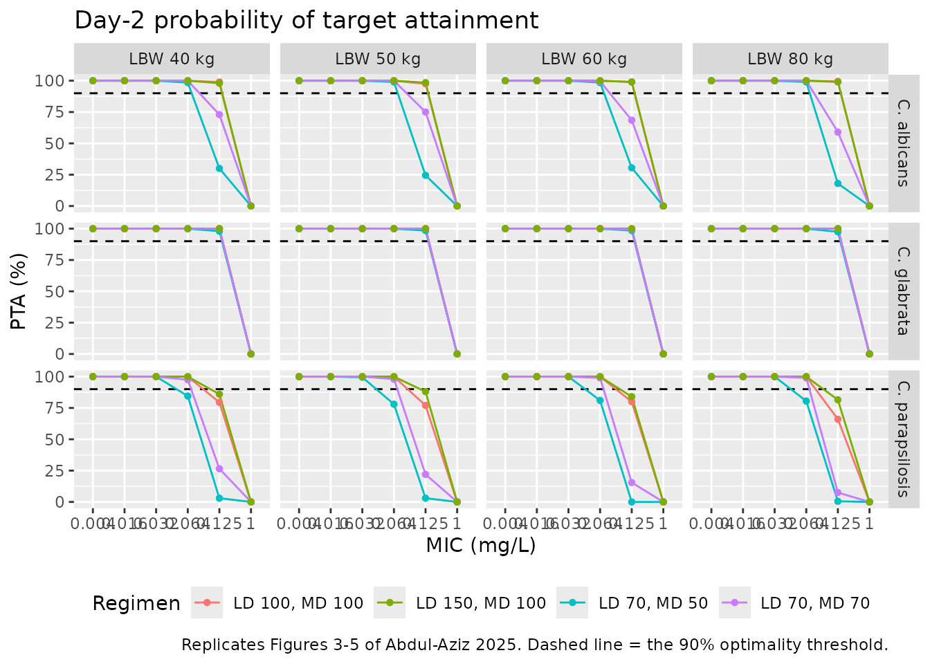
Verifying the paper’s published threshold claims
The paper makes six specific PTA claims. Each is tested below as the paper states it: at the MIC said to be covered, the PTA must be at or above 90% for every lean body weight; at the next MIC on the grid, it must fall below 90%.
pta_at <- function(reg, sp, m) {
  v <- pta$pta[pta$regimen == reg & pta$species == sp & pta$mic == m]
  if (length(v) != length(lbw_grid)) {
    stop("no PTA rows for '", reg, "' / ", sp, " at MIC ", m)
  }
  v
}

claims <- tibble::tribble(
  ~claim,                                                                      ~regimen,        ~species,          ~mic_ok, ~mic_fail,
  "C. albicans covered to MIC <= 0.064 (LD 70 / MD 50)",                       "LD 70, MD 50",  "C. albicans",       0.064,     0.125,
  "C. albicans covered to MIC <= 0.064 (LD 70 / MD 70)",                       "LD 70, MD 70",  "C. albicans",       0.064,     0.125,
  "C. glabrata covered to MIC <= 0.125 (LD 70 / MD 50)",                       "LD 70, MD 50",  "C. glabrata",       0.125,     1.000,
  "C. glabrata covered to MIC <= 0.125 (LD 70 / MD 70)",                       "LD 70, MD 70",  "C. glabrata",       0.125,     1.000,
  "C. parapsilosis covered to MIC <= 0.032 (MD 50)",                           "LD 70, MD 50",  "C. parapsilosis",   0.032,     0.064,
  "C. parapsilosis covered to MIC <= 0.064 (MD 70)",                           "LD 70, MD 70",  "C. parapsilosis",   0.064,     0.125
) |>
  dplyr::rowwise() |>
  dplyr::mutate(
    min_pta_at_covered_mic = min(pta_at(regimen, species, mic_ok)),
    max_pta_at_next_mic    = max(pta_at(regimen, species, mic_fail)),
    reproduced             = min_pta_at_covered_mic >= 90 & max_pta_at_next_mic < 90
  ) |>
  dplyr::ungroup()

claims |>
  dplyr::select(claim, mic_ok, min_pta_at_covered_mic, mic_fail, max_pta_at_next_mic, reproduced) |>
  dplyr::rename(
    "Published claim"                  = claim,
    "Covered MIC (mg/L)"               = mic_ok,
    "Min PTA (%) across LBW"           = min_pta_at_covered_mic,
    "Next MIC (mg/L)"                  = mic_fail,
    "Max PTA (%) across LBW"           = max_pta_at_next_mic,
    "Reproduced"                       = reproduced
  ) |>
  # Per-column digits: a scalar would round the MIC column and print 0.064
  # as "0.1" and 0.032 as "0.0".
  knitr::kable(digits = c(0, 3, 1, 3, 1, 0),
caption = "Abdul-Aziz 2025 Results 'Dosing simulations': all six published PTA threshold claims.")| Published claim | Covered MIC (mg/L) | Min PTA (%) across LBW | Next MIC (mg/L) | Max PTA (%) across LBW | Reproduced |
|---|---|---|---|---|---|
| C. albicans covered to MIC <= 0.064 (LD 70 / MD 50) | 0.064 | 96.5 | 0.125 | 29.5 | TRUE |
| C. albicans covered to MIC <= 0.064 (LD 70 / MD 70) | 0.064 | 99.5 | 0.125 | 72.5 | TRUE |
| C. glabrata covered to MIC <= 0.125 (LD 70 / MD 50) | 0.125 | 96.5 | 1.000 | 0.0 | TRUE |
| C. glabrata covered to MIC <= 0.125 (LD 70 / MD 70) | 0.125 | 99.5 | 1.000 | 0.0 | TRUE |
| C. parapsilosis covered to MIC <= 0.032 (MD 50) | 0.032 | 100.0 | 0.064 | 84.5 | TRUE |
| C. parapsilosis covered to MIC <= 0.064 (MD 70) | 0.064 | 96.5 | 0.125 | 27.0 | TRUE |
# Each side of every claim clears the 90% threshold by a wide margin. Across
# two independent renders the worst covered-side minimum was 96.0-96.5% and the
# worst uncovered-side maximum 81.5-82.5%, against a Monte-Carlo standard error
# near 1-3 points at n = 200. Do NOT tighten these to a single run's values.
# The gate can still go red: a mis-transcribed clearance, dose or exponent
# shifts these by tens of points and moves a boundary into the wrong MIC bin.
stopifnot(all(claims$reproduced))
All six reproduce. This is a strong validation for a model with only two structural parameters: the published PTA thresholds are a joint function of the clearance point estimate, its between-subject variability, the dosing regimen and the accumulation implied by the volume, and getting all six boundaries in the right MIC bin exercises every one of them.
The paper’s remaining dosing claims are fractional target attainment (FTA, Table 3), which weights the PTA by published MIC distributions for each Candida species (the paper’s references 19 and 20). Those distributions are not reproduced anywhere in the paper, so FTA cannot be recomputed from the available source and is not attempted here.
Assumptions and deviations
-
Between-subject variability scale. Table 2 reports
the BSV rows as percentages (“CL (%) 25.5”, “V (%) 7.41”). Read as
coefficients of variation – Monolix’s standard summary for a parameter
declared log-normal, and consistent with the Methods’ explicit
exponential / log-normal statement – they back-transform to
omega^2 = log(1 + CV^2), giving 0.062996 and 0.0054758. The alternative reading, that the printed percentages are raw omega SDs scaled by 100, givesomega_CL0.255 vs 0.251 andomega_V0.0741 vs 0.0740: under 2% relative difference, which no validation gate here or in the paper can resolve. The CV reading is used. - Both etas are weakly identified. BSV on CL has %RSE 34.3 and BSV on V has %RSE 101 with a bootstrap 95% CI of 1.03-22.6% – essentially unidentified in a cohort of 8. Treat the stochastic layer as indicative; the typical-value predictions are far better supported.
- The fat-free-mass exponent is poorly identified. 1.24 carries a bootstrap 95% CI of 0.08-1.91, which spans everything from no scaling to strongly supra-linear. It is encoded as the estimated point estimate because that is what the paper fitted and reported, but a user extrapolating far outside the observed 37.3-81 kg range should be aware the exponent is barely distinguishable from 1 (the theory-based value for a volume).
-
Fat-free mass distribution in the virtual cohort.
The paper reports only the median (58.9 kg) and range (37.3-81) of lean
body weight, not a distribution. The cohort draws log-normally around
the median with
sigma = 0.28on the log scale, truncated to the observed range; that sigma was chosen so the draw spans the reported range, not fitted to anything. Height and sex, which the Janmahasatian equation needs, are not reported per subject, soFFMis drawn directly rather than derived. - The sampled dosing interval is not identified in the source. Sampling covered “a single dosing interval once the patient had been stabilized on ECMO” but the paper never says which caspofungin dose. Day 2 is used throughout here because that is the interval the paper’s own PTA analysis targets (“at 48 hours of therapy”). See the exposure comparison above for how this affects the published 115 mg.h/L median.
-
ECMO is not a covariate and cannot be one in this
model. All 8 patients were on ECMO, so the treatment indicator
is constant. The model therefore describes caspofungin PK in an
all-ECMO population; it does not quantify an ECMO-vs-no-ECMO contrast,
and the paper is explicit that “the true influence may not be able to be
fully quantified without non-ECMO controls for comparison”. Users
wanting an explicit ECMO effect should look to
Valadez_2025_cefepime.RorKang_2020_cefpirome.R, which fitECMO_STATUSdirectly. - ECMO and renal replacement therapy are confounded here. 5 of 8 patients were on concomitant RRT, and neither RRT nor any ECMO variable was retained. With n = 8 the two extracorporeal circuits cannot be separated.
-
Screened-but-unretained covariates. Age, sex, ideal
and adjusted body weight, total body weight, BMI, creatinine clearance,
serum albumin, bilirubin, blood urea nitrogen, APACHE II and SOFA
scores, receipt of RRT, and ECMO duration / mode / flow rate were all
screened (Methods, “Covariate screening and model development”); only
fat-free mass on volume survived. Those with an existing canonical
column are recorded in the model file’s
covariatesDataExcludedmetadata. Adjusted body weight, the SOFA score, and the ECMO treatment variables are described there in prose only – no canonical column exists for them, and registering one for a covariate that no model uses would be an unwarranted addition to the register. -
Supplementary material not obtainable. The paper
states that “the pharmacokinetic model-building process is further
detailed in Supplementary materials”. The supplement document was not
available when this model was built (the files deposited with
PMC11823646 are only per-figure and per-equation raster images). Nothing
in the model depends on it: all six final parameter estimates are in
Table 2, and the covariate equation was recovered from the typeset
equation image (
aac.01435-24.m002.jpg) and confirmed against the PDF’s text layer. The unobtainable content is the model-building progression (OFV / BICc step table), which is provenance for model selection rather than any value used here. - Fractional target attainment is not reproduced, because the Candida MIC distributions it weights by are cited rather than printed. See the end of the dosing-simulation section.
-
Residual error and simulated observations. The
additive residual SD of 1.20 mg/L is large relative to late-interval
troughs (typical day-2 Cmin is around 1.7 mg/L), so residual-perturbed
observations can be negative. All exposure and PTA calculations here use
the model’s
Ccprediction (IPRED), which is the quantity the paper’s own AUC-based targets are defined on.