Isoniazid + acetylisoniazid, NAT2 pharmacogenetics (Chen 2022)
Source:vignettes/articles/Chen_2022_isoniazid.Rmd
Chen_2022_isoniazid.RmdModel and source
- Citation: Chen B, Shi H-Q, Feng MR, Wang X-H, Cao X-M, Cai W-M (2022). Population Pharmacokinetics and Pharmacodynamics of Isoniazid and its Metabolite Acetylisoniazid in Chinese Population. Front Pharmacol 13:932686.
- Article: doi:10.3389/fphar.2022.932686
Chen 2022 built an integrated parent-metabolite population PK model
for oral isoniazid (INH) and its acetylation product acetylisoniazid
(AcINH) in healthy Chinese adults and Chinese tuberculosis patients
(Figure 1 of the paper). INH is a one-compartment model with first-order
absorption (Ka); a fraction FM of INH
clearance forms AcINH, which has its own one-compartment disposition
with a first-order elimination rate constant K30. The
remaining fraction of INH clearance, 1 - FM, and the AcINH
elimination both leave the system.
The N-acetyltransferase 2 (NAT2) genotype was the only retained covariate, and the paper reports two equally final parameterisations of it (Table 3):
-
Final Model (2) – a per-allele model, carried here
as
Chen_2022_isoniazid. The number of each of the NAT2*5,*6and*7slow alleles enters exponentially on bothCL/FandFM. This is the paper’s preferred model: it gave the largest objective-function drop (Delta OFV = -315.5 against -275.3 for the class model). -
Final Model (1) – a three-level genotype-class
model, carried here as
Chen_2022_isoniazid_nat2class. A single class score (0 = wt/wt, 1 = m/wt, 2 = m/m) enters exponentially onCL/FandFM.
mod_allele <- rxode2::rxode2(readModelDb("Chen_2022_isoniazid"))
#> ℹ parameter labels from comments will be replaced by 'label()'
mod_class  <- rxode2::rxode2(readModelDb("Chen_2022_isoniazid_nat2class"))
#> ℹ parameter labels from comments will be replaced by 'label()'
mod_allele
#>  ── rxode2-based free-form 3-cmt ODE model ──────────────────────────────────────
#>  ── Initalization: ──
#> Fixed Effects ($theta):
#>                     lka                     lcl              lkel_acinh
#>               1.3837912               3.4078419              -1.2039728
#>                     lvc               lvc_acinh                     lfm
#>               3.9396382               2.5176965              -0.1508229
#> e_snp_nat2_rs1801280_cl e_snp_nat2_rs1799930_cl e_snp_nat2_rs1799931_cl
#>              -0.7700000              -0.6000000              -0.2900000
#> e_snp_nat2_rs1801280_fm e_snp_nat2_rs1799930_fm e_snp_nat2_rs1799931_fm
#>              -0.7200000              -0.4500000              -0.1400000
#>                  mw_inh                  propSd            propSd_acinh
#>             137.1400000               0.3390000               0.2950000
#>
#> Omega ($omega):
#>                 etalka   etalcl etalkel_acinh   etalvc    etalfm
#> etalka        0.286225 0.000000      0.000000 0.000000 0.0000000
#> etalcl        0.000000 0.078961      0.000000 0.000000 0.0000000
#> etalkel_acinh 0.000000 0.000000      0.048841 0.000000 0.0000000
#> etalvc        0.000000 0.000000      0.000000 0.039204 0.0000000
#> etalfm        0.000000 0.000000      0.000000 0.000000 0.0096432
#> attr(,"lotriLabels")
#> [1] "Table 3 Final Model (2) omega Ka = 53.5 percent; 0.535^2"
#> [2] "Table 3 Final Model (2) omega CL/F = 28.1 percent; 0.281^2"
#> [3] "Table 3 Final Model (2) omega K30 = 22.1 percent; 0.221^2"
#> [4] "Table 3 Final Model (2) omega V2/F = 19.8 percent; 0.198^2"
#> [5] "Table 3 Final Model (2) omega FM = 9.82 percent; 0.0982^2"
#> attr(,"lotriFix")
#>               etalka etalcl etalkel_acinh etalvc etalfm
#> etalka         FALSE  FALSE         FALSE  FALSE  FALSE
#> etalcl         FALSE  FALSE         FALSE  FALSE  FALSE
#> etalkel_acinh  FALSE  FALSE         FALSE  FALSE  FALSE
#> etalvc         FALSE  FALSE         FALSE  FALSE  FALSE
#> etalfm         FALSE  FALSE         FALSE  FALSE  FALSE
#>
#> States ($state or $stateDf):
#>   Compartment Number Compartment Name
#> 1                  1            depot
#> 2                  2          central
#> 3                  3    central_acinh
#>  ── Multiple Endpoint Model ($multipleEndpoint): ──
#>       variable                     cmt                     dvid*
#> 1       Cc ~ …       cmt='Cc' or cmt=4       dvid='Cc' or dvid=1
#> 2 Cc_acinh ~ … cmt='Cc_acinh' or cmt=5 dvid='Cc_acinh' or dvid=2
#>   * If dvids are outside this range, all dvids are re-numered sequentially, ie 1,7, 10 becomes 1,2,3 etc
#>
#>  ── μ-referencing ($muRefTable): ──
#>        theta           eta level
#> 1        lka        etalka    id
#> 2        lcl        etalcl    id
#> 3        lvc        etalvc    id
#> 4 lkel_acinh etalkel_acinh    id
#> 5        lfm        etalfm    id
#>
#>  ── Model (Normalized Syntax): ──
#> function() {
#>     compartmentData <- list(depot = list(analyte = "isoniazid",
#>         units = "mg", specimen = "administration site", verified = TRUE),
#>         central = list(analyte = "isoniazid", units = "mg", specimen = "plasma",
#>             verified = TRUE), central_acinh = list(analyte = "acetylisoniazid",
#>             units = "umol", specimen = "plasma", verified = TRUE))
#>     covariateData <- list(SNP_NAT2_RS1801280_C_COUNT = list(description = "Number of NAT2 *5 alleles (341T>C, rs1801280 variant C allele): 0, 1 or 2.",
#>         units = "(count, 0/1/2 alleles per subject)", type = "continuous",
#>         reference_category = "0 (no *5 allele)", notes = "Chen 2022 Methods 'Covariates' method 3 scores each of the *5, *6 and *7 alleles as 0 (w/w), 1 (m/w) or 2 (m/m); Table 3 row 'M341'. The paper identifies *5 by the 341 SNP alone (allele-specific PCR), so the *5 allele count equals the rs1801280 variant-allele count. The paper writes the SNP as 'C341 -> T'; the NAT2*5 defining change is 341T>C (variant C). Enters as exp(-0.77 * count) on CL/F and exp(-0.72 * count) on FM.",
#>         source_name = "M341"), SNP_NAT2_RS1799930_A_COUNT = list(description = "Number of NAT2 *6 alleles (590G>A, rs1799930 variant A allele): 0, 1 or 2.",
#>         units = "(count, 0/1/2 alleles per subject)", type = "continuous",
#>         reference_category = "0 (no *6 allele)", notes = "Chen 2022 Methods 'Covariates' method 3; Table 3 row 'M590'. Enters as exp(-0.60 * count) on CL/F and exp(-0.45 * count) on FM.",
#>         source_name = "M590"), SNP_NAT2_RS1799931_A_COUNT = list(description = "Number of NAT2 *7 alleles (857G>A, rs1799931 variant A allele): 0, 1 or 2.",
#>         units = "(count, 0/1/2 alleles per subject)", type = "continuous",
#>         reference_category = "0 (no *7 allele)", notes = "Chen 2022 Methods 'Covariates' method 3; Table 3 row 'M870' and the Table 3 footnote 'M803' are both misprints of the 857 position that defines NAT2*7 (Methods 'Genotyping': 'G857 -> A'). Enters as exp(-0.29 * count) on CL/F and exp(-0.14 * count) on FM.",
#>         source_name = "M870"))
#>     description <- "Integrated parent-metabolite population PK model for oral isoniazid (INH) and its metabolite acetylisoniazid (AcINH) in 45 healthy Chinese adults and 157 Chinese adults with tuberculosis (Chen 2022, Final Model (2)). One-compartment INH with first-order absorption; a fraction FM of INH clearance forms AcINH, which has its own one-compartment disposition with first-order elimination rate K30. The numbers of NAT2 *5 (341T>C), *6 (590G>A) and *7 (857G>A) alleles each enter exponentially on INH CL/F and on FM. Concentrations are in umol/L (doses in mg are converted with the INH molecular weight). Known deviation: the printed AcINH parameters (K30 x V3/F = 3.7 L/h) give a typical AcINH exposure about twice the paper's own observed NCA and VPC in NAT2 *4/*4 subjects; INH reproduces. See the vignette."
#>     population <- list(species = "human", n_subjects = 202L,
#>         n_studies = 3L, age_range = "19-64 years (healthy 21-29 years; patients 19-64 years)",
#>         weight_range = "39-78 kg", sex_female_pct = 33.7, race_ethnicity = "Chinese (healthy subjects all Han)",
#>         disease_state = "45 healthy adult male volunteers (two single-dose studies) and 157 adults with pulmonary tuberculosis on 7-14 days of combination therapy (isoniazid with rifampicin or rifapentine, pyrazinamide and ethambutol).",
#>         dose_range = "Healthy: single oral 300 mg (study 1, n = 24) or 320 mg (study 2, bioequivalence, n = 21). Patients: daily oral isoniazid, sampled 2 and/or 6 h post-dose.",
#>         regions = "China", nat2_genotype_counts = c(`*4/*4` = 91L,
#>             `*4/*5` = 7L, `*4/*6` = 43L, `*4/*7` = 29L, `*5/*7` = 3L,
#>             `*6/*6` = 20L, `*6/*7` = 5L, `*7/*7` = 4L), notes = "Table 1 demographics; NAT2 genotype counts summed from Results 'INH and AcINH in Relation to NAT2 Genotypes' over the three cohorts (study 1: 8/0/6/2/1/7/0/0; study 2: 11/1/6/2/0/1/0/0; patients: 72/6/31/25/2/12/5/4 in the order listed). 122 subjects formed the index group and 80 the validation group; the final model was fit to both. Female percentage is 68/202 (all healthy volunteers male).")
#>     reference <- "Chen B, Shi H-Q, Feng MR, Wang X-H, Cao X-M, Cai W-M (2022). Population Pharmacokinetics and Pharmacodynamics of Isoniazid and its Metabolite Acetylisoniazid in Chinese Population. Front Pharmacol 13:932686. doi:10.3389/fphar.2022.932686."
#>     units <- list(time = "h", dosing = "mg", concentration = "umol/L")
#>     vignette <- "Chen_2022_isoniazid"
#>     ini({
#>         lka <- 1.38379123090177
#>         label("INH first-order absorption rate constant Ka (1/h)")
#>         lcl <- 3.40784192438082
#>         label("INH apparent clearance CL/F for NAT2 *4/*4 (L/h)")
#>         lkel_acinh <- -1.20397280432594
#>         label("AcINH elimination rate constant K30 (1/h)")
#>         lvc <- 3.93963817246112
#>         label("INH apparent volume of distribution V2/F (L)")
#>         lvc_acinh <- 2.51769647261099
#>         label("AcINH apparent volume of distribution V3/F (L)")
#>         lfm <- -0.150822889734584
#>         label("Fraction of INH clearance forming AcINH, FM, for NAT2 *4/*4 (fraction)")
#>         e_snp_nat2_rs1801280_cl <- -0.77
#>         label("Exponent of NAT2 *5 allele count on CL/F (per allele)")
#>         e_snp_nat2_rs1799930_cl <- -0.6
#>         label("Exponent of NAT2 *6 allele count on CL/F (per allele)")
#>         e_snp_nat2_rs1799931_cl <- -0.29
#>         label("Exponent of NAT2 *7 allele count on CL/F (per allele)")
#>         e_snp_nat2_rs1801280_fm <- -0.72
#>         label("Exponent of NAT2 *5 allele count on FM (per allele)")
#>         e_snp_nat2_rs1799930_fm <- -0.45
#>         label("Exponent of NAT2 *6 allele count on FM (per allele)")
#>         e_snp_nat2_rs1799931_fm <- -0.14
#>         label("Exponent of NAT2 *7 allele count on FM (per allele)")
#>         mw_inh <- fix(137.14)
#>         label("Isoniazid molecular weight (g/mol)")
#>         propSd <- c(0, 0.339)
#>         label("INH proportional residual error (fraction)")
#>         propSd_acinh <- c(0, 0.295)
#>         label("AcINH proportional residual error (fraction)")
#>         etalka ~ 0.286225
#>         label("Table 3 Final Model (2) omega Ka = 53.5 percent; 0.535^2")
#>         etalcl ~ 0.078961
#>         label("Table 3 Final Model (2) omega CL/F = 28.1 percent; 0.281^2")
#>         etalkel_acinh ~ 0.048841
#>         label("Table 3 Final Model (2) omega K30 = 22.1 percent; 0.221^2")
#>         etalvc ~ 0.039204
#>         label("Table 3 Final Model (2) omega V2/F = 19.8 percent; 0.198^2")
#>         etalfm ~ 0.0096432
#>         label("Table 3 Final Model (2) omega FM = 9.82 percent; 0.0982^2")
#>     })
#>     model({
#>         nat2_cl <- exp(e_snp_nat2_rs1801280_cl * SNP_NAT2_RS1801280_C_COUNT +
#>             e_snp_nat2_rs1799930_cl * SNP_NAT2_RS1799930_A_COUNT +
#>             e_snp_nat2_rs1799931_cl * SNP_NAT2_RS1799931_A_COUNT)
#>         nat2_fm <- exp(e_snp_nat2_rs1801280_fm * SNP_NAT2_RS1801280_C_COUNT +
#>             e_snp_nat2_rs1799930_fm * SNP_NAT2_RS1799930_A_COUNT +
#>             e_snp_nat2_rs1799931_fm * SNP_NAT2_RS1799931_A_COUNT)
#>         ka <- exp(lka + etalka)
#>         cl <- exp(lcl + etalcl) * nat2_cl
#>         vc <- exp(lvc + etalvc)
#>         kel_acinh <- exp(lkel_acinh + etalkel_acinh)
#>         vc_acinh <- exp(lvc_acinh)
#>         fm <- exp(lfm + etalfm) * nat2_fm
#>         kel <- cl/vc
#>         d/dt(depot) <- -ka * depot
#>         d/dt(central) <- ka * depot - kel * central
#>         d/dt(central_acinh) <- fm * kel * central * 1000/mw_inh -
#>             kel_acinh * central_acinh
#>         Cc <- central/vc * 1000/mw_inh
#>         Cc_acinh <- central_acinh/vc_acinh
#>         Cc ~ prop(propSd)
#>         Cc_acinh ~ prop(propSd_acinh)
#>     })
#> }
The paper reported and plotted all concentrations in umol/L. The
model files store doses in mg and convert to umol with the isoniazid
molecular weight (137.14 g/mol), so Cc and
Cc_acinh come out in umol/L to match the paper’s figures
and Table 2.
Population
The analysis pooled 202 subjects across three cohorts (Table 1 and the Results section “INH and AcINH in Relation to NAT2 Genotypes”):
- Study 1 – 24 healthy adult men, single oral 300 mg INH, rich sampling over 0-14 h.
- Study 2 – 21 healthy adults, single oral 320 mg INH (bioequivalence study).
- Patients – 157 adults with pulmonary tuberculosis (89 men, 68 women; mean age 42.2 y, weight 56.5 kg) on 7-14 days of combination therapy, sampled 2 and/or 6 h after a dose.
122 subjects formed the model-building (index) group and 80 the
validation group; the final model was fit to both. Eight NAT2 diplotypes
were observed (*4/*4, *4/*5,
*4/*6, *4/*7, *5/*7,
*6/*6, *6/*7, *7/*7), with
*4/*4 (wild type) the most common.
mod_allele$meta$population[c("n_subjects", "weight_range", "disease_state")]
#> $n_subjects
#> [1] 202
#>
#> $weight_range
#> [1] "39-78 kg"
#>
#> $disease_state
#> [1] "45 healthy adult male volunteers (two single-dose studies) and 157 adults with pulmonary tuberculosis on 7-14 days of combination therapy (isoniazid with rifampicin or rifapentine, pyrazinamide and ethambutol)."
Source trace
Every ini() value is traced to Table 3 of Chen 2022 in
an in-file comment next to the parameter. The table below collects the
structural values of both final models.
| Parameter | Final Model (2) (Chen_2022_isoniazid) |
Final Model (1) (Chen_2022_isoniazid_nat2class) |
Source |
|---|---|---|---|
Ka (1/h) |
3.99 | 3.91 | Table 3 theta1 |
CL/F (L/h), *4/*4
|
30.2 | 28.7 | Table 3 theta2 |
K30 (1/h) |
0.30 | 0.41 | Table 3 theta3 |
V2/F (L) |
51.4 | 54.1 | Table 3 theta4 |
V3/F (L) |
12.4 | 17.2 | Table 3 theta5 |
FM |
0.86 | 0.88 | Table 3 theta6 |
*5 effect on CL/F
|
-0.77 (theta7) | class score -0.55 (theta7) | Table 3 |
*6 effect on CL/F
|
-0.60 (theta8) | – | Table 3 |
*7 effect on CL/F
|
-0.29 (theta9) | – | Table 3 |
*5 effect on FM
|
-0.72 (theta10) | class score -0.47 (theta10) | Table 3 |
*6 effect on FM
|
-0.45 (theta11) | – | Table 3 |
*7 effect on FM
|
-0.14 (theta12) | – | Table 3 |
| INH proportional error | 0.339 | 0.333 | Table 3 sigma INH |
| AcINH proportional error | 0.295 | 0.302 | Table 3 sigma AcINH |
The paper’s Table 3 “M341 / M590 / M870” rows label the
*5 (341T>C), *6 (590G>A) and
*7 (857G>A) allele effects; “M803” in the Final Model
(2) footnote is a misprint of the 857 position given in the Methods
“Genotyping” section. The IIV columns are reported as
omega x 100 (a percentage), so each is squared on the
fraction scale to recover the log-scale variance.
NAT2 covariate effects reproduce the reported fold-changes
The per-allele exponents back-transform directly to the fold-changes
the abstract and Results quote: one copy of *5,
*6 or *7 leaves CL/F at 46.3 %,
54.9 % and 74.8 % of *4/*4, and FM at 48.7 %,
63.8 % and 86.9 %.
allele_cl <- exp(c(`*5` = -0.77, `*6` = -0.60, `*7` = -0.29))
allele_fm <- exp(c(`*5` = -0.72, `*6` = -0.45, `*7` = -0.14))
reported_cl <- c(`*5` = 0.463, `*6` = 0.549, `*7` = 0.748)
reported_fm <- c(`*5` = 0.487, `*6` = 0.638, `*7` = 0.869)

data.frame(
  allele      = names(allele_cl),
  CLF_model   = round(allele_cl, 3),
  CLF_paper   = reported_cl,
  FM_model    = round(allele_fm, 3),
  FM_paper    = reported_fm
)
#>    allele CLF_model CLF_paper FM_model FM_paper
#> *5     *5     0.463     0.463    0.487    0.487
#> *6     *6     0.549     0.549    0.638    0.638
#> *7     *7     0.748     0.748    0.869    0.869

# These are exact algebra (no simulation), so a tight bound is correct here.
stopifnot(
  max(abs(allele_cl - reported_cl)) < 0.005,
  max(abs(allele_fm - reported_fm)) < 0.005
)
The class model’s score coefficient of -0.55 on CL/F
gives the m/wt and m/m CL/F as
exp(-0.55) = 57.7 % and exp(-1.1) = 33.3 % of
wt/wt, consistent with the Results statement that the IIV on
CL/F fell from 56.6 % to 28.1 % once NAT2 was added.
Typical-value isoniazid profiles and NCA
We simulate a single 300 mg oral dose at the typical-value parameters
(no random effects) for the three NAT2 genotype classes and check the
INH NCA against the observed values in Table 2 (healthy wt/wt subjects).
For the per-allele model we use representative diplotypes:
*4/*4 (wt/wt), *4/*6 (one *6,
m/wt) and *6/*6 (two *6, m/m), the most common
mutant alleles in the cohort.
tgrid <- seq(0, 14, by = 0.1)

# Covariate sets for the per-allele model, keyed by genotype class.
allele_cov <- list(
  "wt/wt" = c(0, 0, 0),
  "m/wt"  = c(0, 1, 0),
  "m/m"   = c(0, 2, 0)
)

sim_allele_typ <- function(label, counts) {
  cov <- data.frame(
    SNP_NAT2_RS1801280_C_COUNT = counts[1],
    SNP_NAT2_RS1799930_A_COUNT = counts[2],
    SNP_NAT2_RS1799931_A_COUNT = counts[3]
  )
  dose <- data.frame(id = 1, time = 0, amt = 300, evid = 1L, cmt = "depot")
  obs <- tidyr::expand_grid(id = 1, time = tgrid, cmt = c("Cc", "Cc_acinh")) |>
    dplyr::mutate(amt = NA_real_, evid = 0L)
  ev <- dplyr::bind_rows(dose, obs) |>
    dplyr::arrange(time, cmt) |>
    cbind(cov)
  s <- rxode2::rxSolve(mod_allele, ev, omega = NA, sigma = NA,
                       returnType = "data.frame")
  s |>
    dplyr::distinct(time, .keep_all = TRUE) |>
    dplyr::arrange(time) |>
    dplyr::transmute(genotype = label, time, Cc, Cc_acinh)
}

typ <- dplyr::bind_rows(mapply(sim_allele_typ, names(allele_cov), allele_cov,
                               SIMPLIFY = FALSE))
head(typ)
#>   genotype time       Cc  Cc_acinh
#> 1    wt/wt  0.0  0.00000  0.000000
#> 2    wt/wt  0.1 13.57249  1.516741
#> 3    wt/wt  0.2 21.90503  5.209110
#> 4    wt/wt  0.3 26.76580 10.127079
#> 5    wt/wt  0.4 29.33873 15.648963
#> 6    wt/wt  0.5 30.41582 21.372427
PKNCA on the INH typical-value profiles:
conc_df <- typ |>
  dplyr::filter(!is.na(Cc)) |>
  dplyr::select(id = genotype, time, Cc) |>
  dplyr::mutate(genotype = id)

dose_df <- typ |>
  dplyr::distinct(genotype) |>
  dplyr::mutate(id = genotype, time = 0, amt = 300 / 137.14 * 1000)

conc_obj <- PKNCA::PKNCAconc(
  dplyr::select(conc_df, genotype, id, time, Cc),
  Cc ~ time | genotype + id, concu = "umol/L", timeu = "h"
)
dose_obj <- PKNCA::PKNCAdose(dose_df, amt ~ time | genotype + id, doseu = "umol")

intervals <- data.frame(start = 0, end = Inf,
                        cmax = TRUE, tmax = TRUE,
                        aucinf.obs = TRUE, half.life = TRUE)
nca_inh <- PKNCA::pk.nca(PKNCA::PKNCAdata(conc_obj, dose_obj,
                                          intervals = intervals))
nca_wide <- as.data.frame(nca_inh$result) |>
  dplyr::select(genotype, PPTESTCD, PPORRES) |>
  tidyr::pivot_wider(names_from = PPTESTCD, values_from = PPORRES)
nca_wide
#> # A tibble: 3 × 15
#>   genotype  cmax  tmax tlast clast.obs lambda.z r.squared adj.r.squared
#>   <chr>    <dbl> <dbl> <dbl>     <dbl>    <dbl>     <dbl>         <dbl>
#> 1 m/m       36.8   0.8    14    3.74      0.177     1.000         1.000
#> 2 m/wt      34.1   0.7    14    0.507     0.322     1.000         1.000
#> 3 wt/wt     30.5   0.6    14    0.0134    0.586     1.000         1.000
#> # ℹ 7 more variables: lambda.z.time.first <dbl>, lambda.z.time.last <dbl>,
#> #   lambda.z.n.points <dbl>, clast.pred <dbl>, half.life <dbl>,
#> #   span.ratio <dbl>, aucinf.obs <dbl>
Chen 2022 Table 2 reports the observed INH NCA in the healthy
single-dose study. For wt/wt subjects: Cmax 36.0 umol/L,
AUC 75.5 umol*h/L, t1/2 1.15 h,
CL 30.05 L/h. The typical-value AUC matches to within a few
percent (the AUC0-inf = Dose/CL identity is the
load-bearing structural check), and the terminal half-life is
reproduced. The typical-value Cmax lands below the observed
mean because the authors themselves report the absorption phase was
poorly characterised (“the absorption phase was not effectively
estimated … inaccurate in predicting Ka and Cmax”, Discussion
limitations).
wt <- nca_wide[nca_wide$genotype == "wt/wt", ]
# AUC0-inf = Dose/CL is an identity for a linear model, so a mis-transcribed
# clearance, dose or molecular weight would move this by tens of percent.
stopifnot(abs(wt$aucinf.obs - 75.5) / 75.5 < 0.10)
# Terminal half-life from the structural parameters (ln2 * V2 / CL/F).
stopifnot(abs(wt$half.life - 1.15) / 1.15 < 0.15)
Known deviation: acetylisoniazid exposure in Final Model (2)
The printed Final Model (2) metabolite parameters give an apparent
AcINH clearance of K30 x V3/F = 0.30 x 12.4 = 3.7 L/h. With
that value the typical-value AcINH exposure is about twice the observed
NCA (Table 2 wt/wt: Cmax 32.5 umol/L, AUC
245.4 umolh/L), even though INH reproduces. Final Model (1), whose
K30 x V3/F = 0.41 x 17.2 = 7.1 L/h, reproduces the AcINH
AUC to within ~10 %. The paper’s own Discussion states the AcINH
clearance “was estimated as 11.3 Lh^-1”, which neither printed
K30 x V3/F product equals; the AcINH disposition parameters
are internally inconsistent as printed.
Both models encode exactly what Table 3 reports – no value is tuned. The INH layer, which is what drives the exposure-response / target-attainment analysis in the paper, is sound in both.
acinh_auc <- function(df) {
  d <- dplyr::filter(df, genotype == "wt/wt")
  sum(diff(d$time) * (head(d$Cc_acinh, -1) + tail(d$Cc_acinh, -1)) / 2)
}
sim_class_typ <- function(label, rapid, slow) {
  cov <- data.frame(NAT2_RAPID = rapid, NAT2_SLOW = slow)
  dose <- data.frame(id = 1, time = 0, amt = 300, evid = 1L, cmt = "depot")
  obs <- tidyr::expand_grid(id = 1, time = tgrid, cmt = c("Cc", "Cc_acinh")) |>
    dplyr::mutate(amt = NA_real_, evid = 0L)
  ev <- dplyr::bind_rows(dose, obs) |> dplyr::arrange(time, cmt) |> cbind(cov)
  s <- rxode2::rxSolve(mod_class, ev, omega = NA, sigma = NA,
                       returnType = "data.frame")
  s |> dplyr::distinct(time, .keep_all = TRUE) |> dplyr::arrange(time) |>
    dplyr::transmute(genotype = label, time, Cc, Cc_acinh)
}
typ_class <- dplyr::bind_rows(
  sim_class_typ("wt/wt", 1, 0),
  sim_class_typ("m/wt", 0, 0),
  sim_class_typ("m/m", 0, 1)
)

auc_allele <- acinh_auc(typ)        # Final Model (2)
auc_class  <- acinh_auc(typ_class)  # Final Model (1)
data.frame(
  model = c("Final Model (2) per-allele", "Final Model (1) class"),
  acinh_auc0_14 = round(c(auc_allele, auc_class), 0),
  observed = 245.4
)
#>                        model acinh_auc0_14 observed
#> 1 Final Model (2) per-allele           489    245.4
#> 2      Final Model (1) class           269    245.4

# Final Model (1) reproduces AcINH AUC; Final Model (2) is the ~2x deviation.
# These bounds document the known behaviour; they fail only if a structural
# value (K30, V3/F, FM or the molecular weight) is mis-transcribed.
stopifnot(abs(auc_class - 245.4) / 245.4 < 0.20)
stopifnot(auc_allele / auc_class > 1.5)
Replicating the concentration-time profiles (Figure 4)
Typical-value INH and AcINH profiles by NAT2 genotype class reproduce the shape of Chen 2022 Figure 4: slower INH elimination (and a higher, flatter INH peak) with increasing numbers of slow alleles, and the opposite ordering for AcINH as less INH is acetylated.
plt <- typ |>
  tidyr::pivot_longer(c(Cc, Cc_acinh), names_to = "analyte", values_to = "conc") |>
  dplyr::mutate(analyte = dplyr::recode(analyte, Cc = "INH", Cc_acinh = "AcINH"),
                analyte = factor(analyte, c("INH", "AcINH")),
                genotype = factor(genotype, c("wt/wt", "m/wt", "m/m")))

ggplot(plt, aes(time, conc, colour = genotype)) +
  geom_line(linewidth = 0.8) +
  facet_wrap(~analyte, scales = "free_y") +
  labs(x = "Time (h)", y = "Concentration (umol/L)", colour = "NAT2") +
  theme_bw()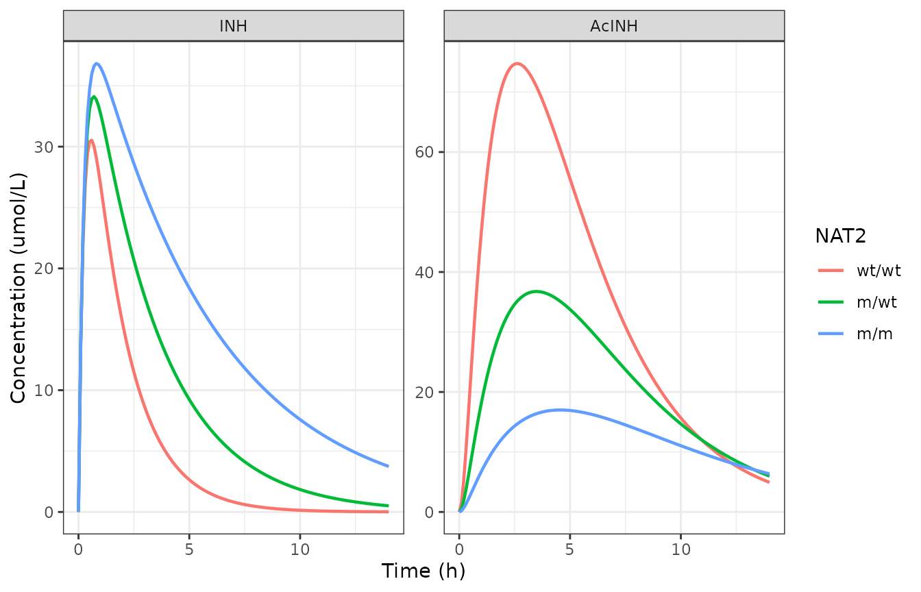
A small stochastic cohort
A 100-subject-per-class stochastic simulation (the full between-subject variability of Final Model (2)) illustrates the spread the VPC in Figure 4 summarises. Residual error is left off so the curves show the structural plus IIV spread.
rxode2::rxSetSeed(1234)
nsub <- 100
sim_cohort <- function(label, counts) {
  cov <- data.frame(
    SNP_NAT2_RS1801280_C_COUNT = counts[1],
    SNP_NAT2_RS1799930_A_COUNT = counts[2],
    SNP_NAT2_RS1799931_A_COUNT = counts[3]
  )
  dose <- tidyr::expand_grid(id = seq_len(nsub), time = 0) |>
    dplyr::mutate(amt = 300, evid = 1L, cmt = "depot")
  obs <- tidyr::expand_grid(id = seq_len(nsub), time = seq(0, 14, by = 0.5),
                            cmt = "Cc") |>
    dplyr::mutate(amt = NA_real_, evid = 0L)
  ev <- dplyr::bind_rows(dose, obs) |>
    dplyr::arrange(id, time) |>
    cbind(cov)
  s <- rxode2::rxSolve(mod_allele, ev, returnType = "data.frame")
  s |> dplyr::mutate(genotype = label)
}
cohort <- dplyr::bind_rows(mapply(sim_cohort, names(allele_cov), allele_cov,
                                  SIMPLIFY = FALSE))

qs <- cohort |>
  dplyr::group_by(genotype = factor(genotype, c("wt/wt", "m/wt", "m/m")), time) |>
  dplyr::summarise(med = median(Cc),
                   lo = quantile(Cc, 0.05),
                   hi = quantile(Cc, 0.95), .groups = "drop")

ggplot(qs, aes(time, med, colour = genotype, fill = genotype)) +
  geom_ribbon(aes(ymin = lo, ymax = hi), alpha = 0.15, colour = NA) +
  geom_line(linewidth = 0.8) +
  labs(x = "Time (h)", y = "INH concentration (umol/L)",
       colour = "NAT2", fill = "NAT2") +
  theme_bw()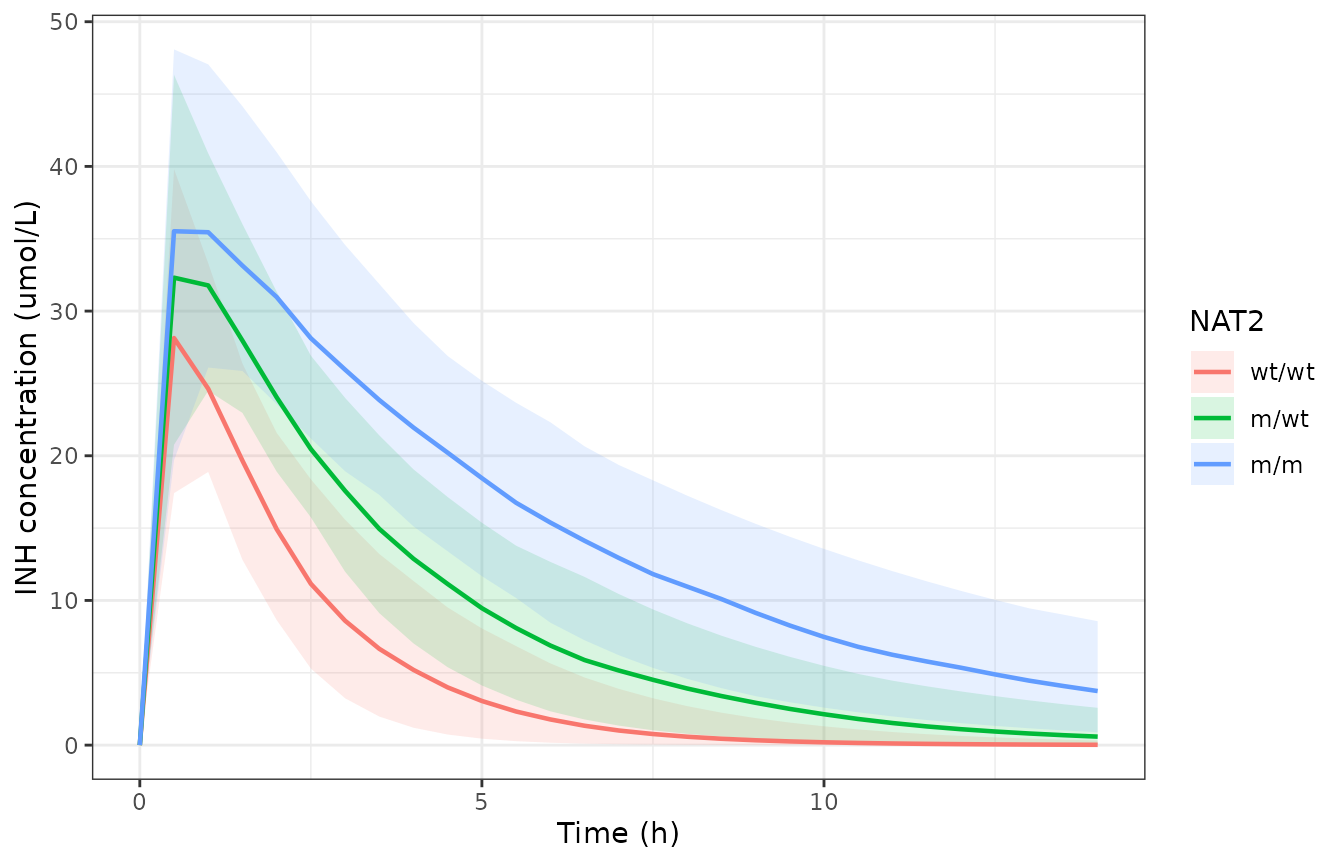
Assumptions and deviations
- Units. The paper plots and tabulates concentrations in umol/L. Doses are carried in mg and converted with the isoniazid molecular weight 137.14 g/mol, which is consistent with the paper’s own unit pairs (e.g. the calibration range 15.89 mg/L = 115.9 umol/L, and 19.7 ugh/mL = 143.4 umolh/L).
-
FMis not bounded above by 1. Chen 2022 uses an exponential covariate modelFM = theta6 * exp(sum thetak * allele)(Eq. 1 / Table 3 footnote), so the wt/wtFMof 0.86-0.88 is a free parameter rather than a logit-constrained fraction. The model encodes it as printed. -
Acetylisoniazid exposure, Final Model (2). As
documented above, the printed Final Model (2)
K30 x V3/Fgives an AcINH exposure about twice the observed NCA, while Final Model (1) reproduces it. Both are faithful transcriptions of Table 3; nothing is tuned. -
Isoniazid Cmax. The typical-value
Cmaxsits below the observed mean because the authors report the absorption phase (and henceKa/Cmax) was poorly estimated from the sparse early sampling. The AUC and terminal half-life, which depend onCL/FandV2/F, are reproduced. -
Genotype representatives. Table 2’s NCA is reported
by genotype class (wt/wt, m/wt, m/m). For the per-allele model these
classes are illustrated with the most common diplotypes
(
*4/*4,*4/*6,*6/*6); other mutant alleles give the per-allele fold-changes verified above. - No weight or renal covariate. Only NAT2 was retained in the final model (Results), so body weight, age, creatinine clearance and the transaminases that were screened do not enter either model. ```