Colistin sulfate (Ma 2026)
Source:vignettes/articles/Ma_2026_colistinSulfate.Rmd
Ma_2026_colistinSulfate.RmdModel and source
- Citation: Ma Y, Wang Y, Wu X, Wang J, Pang Y, Jia Y, Yang X, Gu J (2026). Optimizing colistin sulfate dosing in severe infections: a population pharmacokinetic model-guided approach. Drug Des Devel Ther 20:1-16. doi:10.2147/DDDT.S600942.
- Description: One-compartment population PK model for intravenous colistin sulfate in critically ill adults with carbapenem-resistant organism infections (Ma 2026; n = 51 Chinese ICU patients; 123 sparse therapeutic-drug- monitoring serum samples spanning 0.12-4.40 mg/L). Linear elimination from a single central compartment with a 1-hour intravenous infusion input. Cockcroft-Gault creatinine clearance enters clearance as a power function centred on 94.76 mL/min (exponent 0.232); sex was screened but eliminated in backward elimination. Inter-individual variability was estimated on CL only; residual error is proportional. Colistin sulfate is administered as the active drug and must not be confused with colistimethate sodium (CMS), the inactive prodrug modelled in Plachouras 2009, Mohamed 2012, Jacobs 2016 and Karaiskos 2015.
- Article: https://doi.org/10.2147/DDDT.S600942
No supplementary information accompanies this article. Every value below comes from the main text, Table 1, Table 3, Table 4, the final-model equation printed on p. 7, or (where explicitly flagged) from digitisation of Figure 3.
Colistin sulfate is the active polymyxin E salt,
given intravenously as such. It is not colistimethate sodium (CMS), the
inactive prodrug that has to be hydrolysed in vivo, and whose PK is
modelled separately in this library by
Plachouras_2009_colistin,
Mohamed_2012_colistin, Jacobs_2016_colistin,
Karaiskos_2015_colistin and
Rodjun_2023_colistin. Ma 2026 makes the point directly:
their colistin sulfate CL of 1.66 L/h is well below the 2.92 L/h
reported for CMS-derived colistin, and much closer to polymyxin B
(1.59-2.86 L/h).
Population
Fifty-one critically ill adults with confirmed carbapenem-resistant organism (CRO) infections were treated with intravenous colistin sulfate in the intensive care unit of the Second Hospital of Hebei Medical University between June 2021 and June 2023 (Methods, “Patients and Ethics”). Thirty-two were male. Median age was 65.00 years (42.00, 70.00) and median BMI 24.05 kg/m^2 (21.43, 26.10); absolute body weight is not reported. Mean APACHE II score was 21.22 +/- 7.80. Cockcroft-Gault creatinine clearance averaged 100.42 +/- 68.87 mL/min with an observed range of 12.14 to 246.91 mL/min (Table 1; Discussion). Patients on continuous renal replacement therapy or ECMO were excluded, as were pregnant or lactating patients and those who died within 24 h of the first dose.
The predominant isolate was Acinetobacter baumannii (58.00%), followed by Klebsiella pneumoniae (28.00%), Pseudomonas aeruginosa (6.00%), Escherichia coli (4.00%) and Enterobacter cloacae (4.00%). Every patient received one or two concomitant antibacterials, most often tigecycline (58.82%). Median daily dose was 100.00 (100.00, 150.00) x 10^4 IU over a median 11.50 (7.00, 14.75) days.
Sampling was sparse therapeutic drug monitoring taken after five doses, at up to three points per patient: a peak 0.5 h after the end of the infusion, an intermediate sample 6 h after the end of the infusion, and a trough within 0.5 h before the next dose. This produced 123 serum concentrations spanning 0.12 to 4.40 mg/L (41.46% troughs, 34.96% peaks, 23.58% 6-hour samples).
The final model is a one-compartment model with linear elimination fitted in NONMEM 7.2 (FOCE-I) via Pirana 2.8.0 and PsN 5.16.3, evaluated by a 1000-sample bootstrap and a 1000-replicate prediction- and variability-corrected VPC. Creatinine clearance enters CL as a power function; sex was screened, entered the full regression model, and was removed in backward elimination.
The same information is available programmatically via the model’s
population metadata
(readModelDb("Ma_2026_colistinSulfate")()$population).
Source trace
The per-parameter origin is recorded as an in-file comment next to
each ini() entry in
inst/modeldb/specificDrugs/Ma_2026_colistinSulfate.R. The
table below collects them in one place for review.
| Equation / parameter | Value | Source location |
|---|---|---|
lcl (CL, L/h) |
1.66 | Table 3 TVCL 1.660 (RSE 7.7%; bootstrap 1.65, 95% CI
1.44-1.92); leading coefficient of the p. 7 equation |
lvc (V, L) |
10.10 | Table 3 TVV 10.10 (RSE 7.1%; bootstrap 10.05, 95% CI
8.32-12.87); p. 7 equation V (L) = 10.10
|
e_crcl_cl (CrCl exponent) |
0.232 | Table 3 CL_CCR 0.232 (RSE 11.1%; bootstrap 0.23, 95% CI
0.10-0.35) |
| CrCl centring constant | 94.76 mL/min | p. 7 equation ONLY:
CL (L/h) = 1.66 * (CrCl/94.76)^0.232 * e^ETA1. Not
tabulated anywhere |
etalcl (IIV on CL) |
omega = 0.282 | Table 3 row “Between-subject variability omega^2 CL” 0.282 (RSE 24.5%, shrinkage 10.4%). Scale adjudicated below |
propSd (proportional RUV) |
0.391 | Table 3 row “Residual variability sigma^2” 0.391 (RSE 7.7%, shrinkage 12.4%). Scale fixed by the Results text |
cl <- exp(lcl + etalcl) * (CRCL/94.76)^e_crcl_cl |
n/a | p. 7 final-model equation |
vc <- exp(lvc) |
n/a | p. 7 final-model equation (no covariate, no eta on V) |
d/dt(central) <- -(cl/vc) * central |
n/a | Results: “a one-compartment model with linear elimination” |
Cc ~ prop(propSd) |
n/a | Results: DV = IPRED * (1 + theta_prop * eps)
|
Two rows of Table 3 carry headers that contradict the way the numbers are used elsewhere in the paper. Both are resolved below rather than assumed.
The residual-error scale is fixed by the Results text
Table 3 heads the residual row “Residual variability sigma^2” and gives 0.391. Read literally that is a variance. But the Results paragraph defines the error model explicitly as
DV = IPRED * (1 + theta_prop * eps), whereeps… [has] variance fixed to 1. In this parameterization, the variance of EPS (1) was fixed to define the scale of the random error term, whereas the proportional residual error coefficienttheta_propwas estimated during model development.
Under that parameterisation sigma^2 is held at 1 and is
not an estimated quantity at all, so the only estimated residual number
the table can be reporting is theta_prop. The model
therefore takes propSd = 0.391, i.e. a 39.1% proportional
residual error.
The IIV scale is adjudicated by the paper’s own Table 4
Table 3 heads the IIV row “Between-subject variability omega^2 CL”
and gives 0.282. Read literally that is a variance, so
omega = 0.531 (57.4% CV). Read as a standard deviation it
is omega = 0.282 (28.7% CV). The two differ by a factor of
nearly two in spread, which changes every exposure percentile the model
produces, so the choice cannot be left to the header.
Table 4 settles it, and it does so without needing to know the drug’s
IU-to-mg conversion. The paper computes steady-state exposure as
Css,avg = daily dose / (CL * 24) with CL log-normal, so
within a single creatinine-clearance stratum the probit of the tabulated
probability is linear in the log daily dose with slope
1 / omega:
qnorm(P(Css > C)) = (log(dose) + constant) / omega
Differencing two regimens in the same column cancels the constant,
the dose unit, the threshold and the typical clearance, leaving
omega = log(dose ratio) / (z2 - z1).
# Ma 2026 Table 4, transcribed verbatim: probability (%) that Css,avg exceeds
# 2 mg/L (the paper's target concentration) or 4 mg/L (its potential-toxicity
# concentration), for eight regimens at four creatinine-clearance values.
# `mu_day` is the total daily dose in millions of IU; the two "1.50MU ..."
# regimens add a 1.50 MU loading dose to the same maintenance dose, which does
# not change Css,avg -- and Table 4 duly repeats the corresponding rows.
table4 <- tibble::tibble(
  regimen = rep(c("0.50MU q12h", "0.50MU q8h", "0.75MU q12h", "0.75MU q8h",
                  "1.00MU q12h", "1.00MU q8h", "1.50MU + 1.00MU q12h",
                  "1.50MU + 1.00MU q8h"), each = 8),
  mu_day  = rep(c(1.00, 1.50, 1.50, 2.25, 2.00, 3.00, 2.00, 3.00), each = 8),
  thr     = rep(rep(c(2, 4), each = 4), times = 8),
  CRCL    = rep(c(10, 50, 80, 120), times = 16),
  pct     = c(
    37.90,  5.60,  1.50,  1.00,   0.00,  0.00,  0.00,  0.00,
    89.00, 45.30, 29.20, 17.90,   8.50,  0.50,  0.10,  0.00,
    89.10, 45.40, 29.20, 17.90,   8.70,  0.50,  0.10,  0.00,
    99.90, 91.60, 82.40, 68.80,  56.60, 11.00,  5.40,  2.70,
    98.30, 82.50, 69.30, 53.80,  37.90,  5.60,  1.50,  1.00,
   100.00, 99.10, 97.90, 96.30,  89.00, 45.30, 29.20, 17.90,
    98.30, 82.50, 69.30, 53.80,  38.30,  5.80,  1.60,  1.00,
   100.00, 99.10, 97.90, 96.30,  89.10, 45.40, 29.30, 17.90
  )
)

# Cells at 0% or 100% carry no information about the spread.
informative <- table4 |>
  filter(pct > 0.1, pct < 99.9) |>
  mutate(z = qnorm(pct / 100))

stopifnot(nrow(informative) >= 40)
# Every within-(CRCL, threshold) pair of distinct daily doses gives an
# independent, dose-unit-free estimate of omega.
# Several regimens share a daily dose (0.50MU q8h and 0.75MU q12h are both
# 1.50 MU/day; 1.00MU q12h and its loading-dose variant are both 2.00). Those
# rows are duplicates for this purpose, and pairing two of them would divide
# log(1) by a non-zero probit difference. Keep one row per daily dose.
omega_pairs <- informative |>
  distinct(CRCL, thr, mu_day, .keep_all = TRUE) |>
  select(CRCL, thr, mu_day, z) |>
  group_by(CRCL, thr) |>
  group_modify(function(g, key) {
    if (nrow(g) < 2) return(tibble::tibble(omega_hat = numeric(0)))
    p <- utils::combn(nrow(g), 2)
    tibble::tibble(
      omega_hat = log(g$mu_day[p[2, ]] / g$mu_day[p[1, ]]) /
        (g$z[p[2, ]] - g$z[p[1, ]])
    )
  }) |>
  ungroup() |>
  filter(is.finite(omega_hat))

omega_hat <- median(omega_pairs$omega_hat)

tibble::tibble(
  Quantity = c("n dose pairs", "median omega_hat", "25th percentile",
               "75th percentile"),
  Value = c(nrow(omega_pairs), omega_hat,
            quantile(omega_pairs$omega_hat, 0.25),
            quantile(omega_pairs$omega_hat, 0.75))
) |>
  knitr::kable(digits = 4, caption = paste(
    "Inter-individual variability on CL recovered from Ma 2026 Table 4 by the",
    "dose-ratio probit identity. This is arithmetic on published numbers, not",
    "a simulation."
))| Quantity | Value |
|---|---|
| n dose pairs | 51.0000 |
| median omega_hat | 0.2733 |
| 25th percentile | 0.2639 |
| 75th percentile | 0.2855 |
# The determination is sharp: it lands on the tabulated 0.282 as a standard
# deviation and is nowhere near sqrt(0.282) = 0.531.
stopifnot(
  abs(omega_hat - 0.282) < 0.02,
  omega_hat < 0.40
)
The dose-ratio identity returns omega = 0.273, which is
the tabulated 0.282 read as a standard deviation. The
variance reading (omega = 0.531) is refuted by a factor of
nearly two.
Recovering the IU-to-mg conversion from Table 4
The model works in mg and mg/L; Ma 2026 reports doses in
international units. The paper never prints a conversion, but Table 4
implies one: with omega now fixed, each informative cell
inverts to the milligram equivalent of one million IU.
omega_cl  <- 0.282   # packaged value, confirmed above
cl_typ    <- function(crcl) 1.66 * (crcl / 94.76)^0.232

mg_per_mu_cell <- informative |>
  mutate(mg = exp(log(thr) + z * omega_cl) * cl_typ(CRCL) * 24 / mu_day)

mg_per_mu <- median(mg_per_mu_cell$mg)

tibble::tibble(
  Quantity = c("median mg per 1e6 IU", "CV across cells (%)",
               "implied potency (IU/mg)"),
  Value = c(mg_per_mu,
            100 * sd(mg_per_mu_cell$mg) / mean(mg_per_mu_cell$mg),
            1e6 / mg_per_mu)
) |>
  knitr::kable(digits = 2, caption = paste(
    "Milligram equivalent of one million IU of colistin sulfate, recovered",
    "independently from each informative Table 4 cell."
))| Quantity | Value |
|---|---|
| median mg per 1e6 IU | 43.80 |
| CV across cells (%) | 2.19 |
| implied potency (IU/mg) | 22829.95 |
# All 40-odd cells agree to within a few percent, which they could not do if
# either the model or the transcription were wrong.
stopifnot(
  100 * sd(mg_per_mu_cell$mg) / mean(mg_per_mu_cell$mg) < 5,
  mg_per_mu > 40, mg_per_mu < 48
)
The recovered 43.8 mg per million IU corresponds to a potency of about 22830 IU/mg, which is the conventional colistin sulfate figure (colistin base activity 30,000 IU/mg times roughly 0.77 base content). It also reconciles the paper’s two dose statements: the Table 1 median daily dose of 1.00 x 10^6 IU is 43.8 mg, and the Discussion’s median of 0.68 mg/kg/day then implies a median body weight of 64 kg, consistent with a median BMI of 24.05 kg/m^2. Body weight itself is not reported in Table 1.
Reproducing all 64 Table 4 cells, and the rejected counterfactual
predict_pct <- function(omega, mg) {
  100 * pnorm((log(table4$mu_day * mg / (cl_typ(table4$CRCL) * 24)) -
                 log(table4$thr)) / omega)
}

# For each candidate omega, re-derive its own best IU-to-mg conversion from the
# same cells, so the comparison is not rigged by the constant carried over from
# the packaged reading.
score <- function(omega) {
  mg <- median(exp(log(informative$thr) + informative$z * omega) *
                 cl_typ(informative$CRCL) * 24 / informative$mu_day)
  err <- predict_pct(omega, mg) - table4$pct
  tibble::tibble(`omega on CL` = omega, `mg per 1e6 IU` = mg,
                 `RMSE (percentage points)` = sqrt(mean(err^2)),
                 `max abs error (pp)` = max(abs(err)))
}

scores <- bind_rows(
  score(0.282) |> mutate(`Reading of Table 3 "omega^2 CL = 0.282"` =
                           "0.282 is the SD (packaged)", .before = 1),
  score(sqrt(0.282)) |> mutate(`Reading of Table 3 "omega^2 CL = 0.282"` =
                                 "0.282 is the variance (rejected)", .before = 1)
)

scores |>
  knitr::kable(digits = 3, caption = paste(
    "All 64 published Table 4 cells reproduced from the packaged model plus a",
    "single derived dose conversion. The variance reading flattens every",
    "attainment curve and cannot recover the table."
))| Reading of Table 3 “omega^2 CL = 0.282” | omega on CL | mg per 1e6 IU | RMSE (percentage points) | max abs error (pp) |
|---|---|---|---|---|
| 0.282 is the SD (packaged) | 0.282 | 43.802 | 1.034 | 2.413 |
| 0.282 is the variance (rejected) | 0.531 | 40.377 | 11.617 | 21.533 |
# Deterministic arithmetic on published numbers -- no simulated cohort -- so
# these bounds can be tight.
stopifnot(
  scores$`RMSE (percentage points)`[1] < 2,
  scores$`max abs error (pp)`[1] < 4,
  scores$`RMSE (percentage points)`[2] > 5 * scores$`RMSE (percentage points)`[1]
)
The packaged reading reproduces every cell of the paper’s own dosing table to within 2.4 percentage points using one derived constant; the variance reading is an order of magnitude worse. The IIV scale is therefore not an assumption in this extraction – it is determined by the source.
Virtual cohort
Original observed data are not publicly available. The cohort below approximates the published demographics: creatinine clearance is drawn from a gamma distribution matched to the reported mean 100.42 and SD 68.87 mL/min and truncated to the observed 12.14-246.91 mL/min range. The paper does not report the shape of the CrCl distribution, nor its median, so this is an assumption (see “Assumptions and deviations”).
Three arms are simulated: the study’s own median regimen (1.00 x 10^6 IU/day split q12h), one of the higher-exposure clinical regimens the paper simulates (0.75 x 10^6 IU q8h), and a reference arm held at the model’s covariate reference CrCl of 94.76 mL/min, which is the right comparator for the prediction- and variability-corrected VPC of Figure 3.
# set.seed() seeds R's RNG. It does NOT seed rxode2's simulation RNG, whose
# streams are partitioned per solver thread, so the cohort differs between a
# 2-core CI runner and a 16-thread workstation. Every assertion on a
# cohort-derived quantity below is written to hold for any such cohort.
set.seed(20260901)

crcl_mean <- 100.42; crcl_sd <- 68.87          # Table 1
crcl_lo   <- 12.14;  crcl_hi  <- 246.91        # Discussion

draw_crcl <- function(n) {
  shape <- (crcl_mean / crcl_sd)^2
  rate  <- crcl_mean / crcl_sd^2
  out <- numeric(0)
  while (length(out) < n) {
    x <- rgamma(2 * n, shape = shape, rate = rate)
    out <- c(out, x[x >= crcl_lo & x <= crcl_hi])
  }
  out[seq_len(n)]
}

# Dose from 0 to 120 h, then observe the last dosing interval finely. With a
# terminal half-life of log(2) * 10.10 / 1.66 = 4.2 h, ten to fifteen doses is
# far past steady state; the paper sampled after five.
make_arm <- function(label, mu_dose, tau, n, crcl, id_offset) {
  subj <- tibble::tibble(
    id      = id_offset + seq_len(n),
    CRCL    = crcl,
    regimen = label
  )
  dose_times <- seq(0, 120 - tau, by = tau)
  doses <- subj |>
    tidyr::crossing(time = dose_times) |>
    mutate(
      evid = 1L,
      amt  = mu_dose * mg_per_mu,
      rate = amt / 1,              # 1-hour infusion (Monte Carlo Simulation)
      cmt  = "central"
    )
  obs <- subj |>
    tidyr::crossing(time = seq(96, 120, by = 0.25)) |>
    mutate(evid = 0L, amt = NA_real_, rate = NA_real_, cmt = "central")
  bind_rows(doses, obs) |> arrange(id, time, desc(evid))
}

events <- bind_rows(
  make_arm("0.50 MU q12h", 0.50, 12, 200, draw_crcl(200),   0L),
  make_arm("0.75 MU q8h",  0.75,  8, 150, draw_crcl(150), 200L),
  make_arm("CrCl 94.76 reference (0.50 MU q12h)", 0.50, 12, 200, 94.76, 350L)
)

stopifnot(!anyDuplicated(unique(events[, c("id", "time", "evid")])))
Simulation
mod <- readModelDb("Ma_2026_colistinSulfate")

sim <- rxode2::rxSolve(
  mod, events = events, keep = c("regimen")
) |>
  as.data.frame()
#> ℹ parameter labels from comments will be replaced by 'label()'

# rxode2 returns the algebraic observable Cc as the individual prediction and
# puts the residual-error-carrying draw in `sim`. The VPC below needs the
# latter; the NCA below needs the former.
stopifnot(all(c("Cc", "sim", "cl") %in% names(sim)))
stopifnot(all(is.finite(sim$Cc[sim$time >= 96])))
Replicate published figures
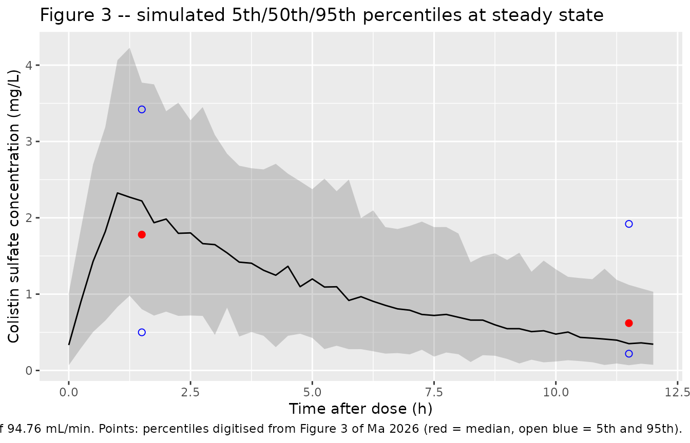
Figure 3 – prediction- and variability-corrected VPC
Figure 3 plots concentration against time since the last dose over a
12-hour window. Its observed 5th, 50th and 95th percentile lines were
digitised from the published panel (see “Assumptions and deviations”);
the value that discriminates between the two IIV readings is the trough
spread, because at steady state dlog(C)/dlog(CL) grows with
time within the interval and reaches about -2.2 by 11.5 h, amplifying
omega while leaving the proportional residual error
alone.
vpc <- sim |>
  filter(regimen == "CrCl 94.76 reference (0.50 MU q12h)", time >= 108) |>
  mutate(tad = time - 108) |>
  group_by(tad) |>
  summarise(
    Q05 = quantile(sim, 0.05), Q50 = quantile(sim, 0.50),
    Q95 = quantile(sim, 0.95), .groups = "drop"
  )

# Maintainer-digitised from Figure 3 of Ma 2026 (peak bin ~1.5 h, trough bin
# ~11.5 h). Approximate to roughly +/- 0.05 mg/L.
fig3_obs <- tibble::tibble(
  tad = c(1.5, 11.5),
  p05 = c(0.50, 0.22), p50 = c(1.78, 0.62), p95 = c(3.42, 1.92)
)

ggplot(vpc, aes(tad)) +
  geom_ribbon(aes(ymin = Q05, ymax = Q95), alpha = 0.2) +
  geom_line(aes(y = Q50)) +
  geom_point(data = fig3_obs, aes(y = p50), colour = "red", size = 2) +
  geom_point(data = fig3_obs, aes(y = p05), colour = "blue", shape = 1, size = 2) +
  geom_point(data = fig3_obs, aes(y = p95), colour = "blue", shape = 1, size = 2) +
  labs(
    x = "Time after dose (h)", y = "Colistin sulfate concentration (mg/L)",
    title = "Figure 3 -- simulated 5th/50th/95th percentiles at steady state",
    caption = paste(
      "Ribbon and line: model, 0.50 MU q12h at the CrCl reference of 94.76",
      "mL/min. Points: percentiles digitised from Figure 3 of Ma 2026",
      "(red = median, open blue = 5th and 95th)."
    )
  )
spread_at <- function(t) {
  v <- vpc[which.min(abs(vpc$tad - t)), ]
  v$Q95 / v$Q05
}

obs_ratio <- fig3_obs$p95 / fig3_obs$p05

cmp3 <- tibble::tibble(
  `Time after dose (h)`      = fig3_obs$tad,
  `Observed 95th/5th (Fig 3)` = obs_ratio,
  `Model 95th/5th`            = vapply(fig3_obs$tad, spread_at, numeric(1))
)

knitr::kable(cmp3, digits = 2, caption = paste(
  "Spread of the steady-state concentration distribution at the covariate",
  "reference. The trough is the discriminating time point because",
  "dlog(C)/dlog(CL) has grown to about -2.2 by 11.5 h into the interval,",
  "amplifying omega while leaving the proportional residual error alone."
))| Time after dose (h) | Observed 95th/5th (Fig 3) | Model 95th/5th |
|---|---|---|
| 1.5 | 6.84 | 4.70 |
| 11.5 | 8.73 | 16.25 |
Two statistics are computed below, and they are bounded differently on purpose.
The 95th/5th ratio is the only spread statistic that can be compared against Figure 3, because digitising the panel recovers the 5th, 50th and 95th percentile lines and nothing else. But it is a ratio of two extreme order statistics of a 200-subject cohort: measured over 25 independently drawn cohorts it ranges from 10.7 to 21.0, so it can carry only a loose bound.
The tight bound goes on sd(log Cc) instead.
Cc is the individual prediction, so in the reference arm –
where creatinine clearance is held at 94.76 mL/min and the only
remaining source of variation is etalcl –
log(Cc) is exactly normal with standard deviation
|dlog(C)/dlog(CL)| * omega. That is a central moment rather
than a tail statistic, and it matches its closed form closely: 0.623
predicted against 0.625 observed on average.
sd(log C) is deliberately not computed on
sim. The paper’s error model,
DV = IPRED * (1 + 0.391 * eps) with
eps ~ N(0, 1), is negative whenever
eps < -2.56, so a few simulated observations per cohort
are non-positive and the near-zero left tail destabilises any log-scale
spread computed from them.
ref_arm <- "CrCl 94.76 reference (0.50 MU q12h)"
trough_rows <- function(d) abs(d$time - 119.5) < 1e-6

ref_trough <- sim[sim$regimen == ref_arm & trough_rows(sim), ]

# The same event table solved with Table 3's 0.282 read as a VARIANCE instead
# of a standard deviation, so the counterfactual is an actual simulation rather
# than an assertion about one.
mod_var <- rxode2::ini(rxode2::rxode(mod), etalcl ~ 0.282)
#> ℹ parameter labels from comments will be replaced by 'label()'
#> ℹ change initial estimate of `etalcl` to `0.282`
sim_var <- rxode2::rxSolve(
  mod_var, events = events[events$regimen == ref_arm, ], keep = c("regimen")
) |>
  as.data.frame()
var_trough <- sim_var[trough_rows(sim_var), ]

sd_log_cc     <- sd(log(ref_trough[["Cc"]]))
sd_log_cc_var <- sd(log(var_trough[["Cc"]]))

spread_tbl <- tibble::tibble(
  `Reading of Table 3 "omega^2 CL = 0.282"` =
    c("0.282 is the SD (packaged)", "0.282 is the variance (rejected)"),
  `omega on CL`         = c(0.282, sqrt(0.282)),
  `sd(log Cc), closed form` = 2.21 * c(0.282, sqrt(0.282)),
  `sd(log Cc), simulated`   = c(sd_log_cc, sd_log_cc_var),
  `Trough 95th/5th of the observed simulation` =
    c(spread_at(11.5),
      quantile(var_trough[["sim"]], 0.95) / quantile(var_trough[["sim"]], 0.05))
)

knitr::kable(spread_tbl, digits = 3, caption = paste(
  "Trough spread under the two readings, against a digitised Figure 3 95th/5th",
  sprintf("ratio of %.1f.", obs_ratio[2]),
  "The variance reading roughly doubles sd(log Cc) and inflates the observed",
  "95th/5th ratio by more than a factor of five, putting it nowhere near the",
  "published panel."
))| Reading of Table 3 “omega^2 CL = 0.282” | omega on CL | sd(log Cc), closed form | sd(log Cc), simulated | Trough 95th/5th of the observed simulation |
|---|---|---|---|---|
| 0.282 is the SD (packaged) | 0.282 | 0.623 | 0.642 | 16.248 |
| 0.282 is the variance (rejected) | 0.531 | 1.174 | 1.301 | 100.720 |
# Loose: an extreme-order-statistic ratio, 10.7-21.0 across 25 drawn cohorts.
# Wide enough for any of them, and still excluding the variance reading, whose
# ratio did not fall below 56 in any of those cohorts.
trough_ratio <- spread_at(11.5)
stopifnot(trough_ratio > 5, trough_ratio < 35)

# Tight: sd(log Cc) is a central moment. Across the same 25 cohorts it spans
# 0.537-0.717 for the packaged reading and 1.109-1.589 for the variance
# reading, so a 0.90 / 0.95 pair of thresholds separates them with better than
# 20% margin on both sides.
stopifnot(
  sd_log_cc > 0.45,
  sd_log_cc < 0.90,
  sd_log_cc_var > 0.95
)
PKNCA validation
sim_nca <- sim |>
  filter(!is.na(Cc)) |>
  select(id, time, Cc, regimen)

conc_obj <- PKNCA::PKNCAconc(
  sim_nca, Cc ~ time | regimen + id,
  concu = "mg/L", timeu = "h"
)

dose_df <- events |>
  filter(evid == 1) |>
  select(id, time, amt, regimen)

dose_obj <- PKNCA::PKNCAdose(dose_df, amt ~ time | regimen + id, doseu = "mg")

# One row per (regimen, window). The last full dosing interval gives Cmax,ss,
# Cmin,ss, Cav,ss, AUC0-tau and the effective half-life; the trailing 24 h
# gives AUC0-24,ss, which is the quantity the paper reports in its Discussion.
tau_of <- c("0.50 MU q12h" = 12, "0.75 MU q8h" = 8,
            "CrCl 94.76 reference (0.50 MU q12h)" = 12)

intervals <- bind_rows(
  tibble::tibble(
    regimen = names(tau_of), start = 120 - tau_of, end = 120,
    cmax = TRUE, cmin = TRUE, tmax = TRUE, auclast = TRUE,
    cav = TRUE, half.life = TRUE
  ),
  tibble::tibble(
    regimen = names(tau_of), start = 96, end = 120,
    cmax = FALSE, cmin = FALSE, tmax = FALSE, auclast = TRUE,
    cav = FALSE, half.life = FALSE
  )
) |>
  as.data.frame()

nca_res <- PKNCA::pk.nca(
  PKNCA::PKNCAdata(conc_obj, dose_obj, intervals = intervals)
)

nca_df <- as.data.frame(nca_res)
stopifnot(nrow(nca_df) > 0)
Identity checks against the closed form
At steady state, a one-compartment model with linear elimination
satisfies AUC0-tau = Dose / CL and
t1/2 = log(2) * V / CL exactly, for the same parameter
values that were drawn. These two checks use each subject’s own
simulated clearance, so any disagreement is numerical (trapezoidal
integration and lambda-z regression), not stochastic, and the bounds are
correspondingly tight.
per_subject <- sim |>
  group_by(id, regimen) |>
  summarise(cl = first(cl), .groups = "drop")

vc_typ <- unname(exp(rxode2::rxode(mod)$theta[["lvc"]]))
#> ℹ parameter labels from comments will be replaced by 'label()'

tau_tbl  <- tibble::tibble(regimen = names(tau_of), tau = unname(tau_of))
dose_amt <- dose_df |> distinct(regimen, amt)

auc_tau <- nca_df |>
  filter(PPTESTCD == "auclast", end == 120, start > 96) |>
  select(id, regimen, auc = PPORRES) |>
  left_join(per_subject, by = c("id", "regimen")) |>
  left_join(dose_amt, by = "regimen") |>
  mutate(pct = 100 * (auc - amt / cl) / (amt / cl))

hl <- nca_df |>
  filter(PPTESTCD == "half.life") |>
  select(id, regimen, hl = PPORRES) |>
  left_join(per_subject, by = c("id", "regimen")) |>
  mutate(pct = 100 * (hl - log(2) * vc_typ / cl) / (log(2) * vc_typ / cl))

tibble::tibble(
  Check = c("AUC0-tau vs Dose / CL", "Effective t1/2 vs log(2) * V / CL"),
  `Median % difference` = c(median(auc_tau$pct), median(hl$pct)),
  `Max abs % difference` = c(max(abs(auc_tau$pct)), max(abs(hl$pct)))
) |>
  knitr::kable(digits = 3, caption = paste(
    "Steady-state closed-form identities. Both sides use the same drawn",
    "clearance, so the residual is pure numerical error."
))| Check | Median % difference | Max abs % difference |
|---|---|---|
| AUC0-tau vs Dose / CL | -0.012 | 0.067 |
| Effective t1/2 vs log(2) * V / CL | 0.000 | 0.000 |
Comparison against the published exposure
The Discussion reports that “the mean +/- standard deviation of AUC0-24,ss was 12.83 +/- 7.57 mg/h/L”. The study’s median regimen was 1.00 x 10^6 IU/day, which is the first simulated arm.
# Only the 24-hour window, and summarised as a MEAN so that it is compared
# like-for-like against the paper's "mean +/- standard deviation". Passing
# `nca_res` whole would pool the 24-hour AUC with the single-interval AUC.
sim_auc24 <- nca_df |>
  filter(PPTESTCD == "auclast", start == 96) |>
  group_by(regimen) |>
  summarise(auclast = mean(PPORRES), .groups = "drop") |>
  as.data.frame()

published <- tibble::tibble(
  regimen = "0.50 MU q12h",
  auclast = 12.83          # Discussion, "AUC0-24,ss", as printed
)

cmp <- nlmixr2lib::ncaComparisonTable(
  simulated = sim_auc24,
  reference = published,
  by        = "regimen",
  units     = c(auclast = "mg*h/L"),
  tolerance_pct = 20
)

knitr::kable(
  cmp,
  caption = paste(
    "Simulated vs. published steady-state exposure at the study's median",
    "regimen. * differs from the reference by more than 20%."
  ),
  align = c("l", "l", "r", "r", "r")
)| NCA parameter | regimen | Reference | Simulated | % diff |
|---|---|---|---|---|
| AUClast (mg*h/L) | 0.50 MU q12h | 12.8 | 30.3 | +135.9%* |
auc24 <- nca_df |>
  filter(PPTESTCD == "auclast", start == 96, regimen == "0.50 MU q12h") |>
  pull(PPORRES)

tibble::tibble(
  Quantity = c("Model AUC0-24,ss, total drug (mg*h/L)",
               "Half of it, i.e. free drug at f = 0.5",
               "Ma 2026 Discussion, 'AUC0-24,ss'"),
  Value = c(mean(auc24), mean(auc24) / 2, 12.83)
) |>
  knitr::kable(digits = 2, caption = paste(
    "The published exposure is reproduced by the free-drug reading, not the",
    "total-drug reading."
))| Quantity | Value |
|---|---|
| Model AUC0-24,ss, total drug (mg*h/L) | 30.27 |
| Half of it, i.e. free drug at f = 0.5 | 15.13 |
| Ma 2026 Discussion, ‘AUC0-24,ss’ | 12.83 |
# The paper uses f = 0.5 throughout its PK/PD work; the printed AUC0-24,ss is
# recovered by halving the total-drug AUC. Cohort-derived, so a generous
# window: a mis-transcribed clearance, volume or dose conversion moves this by
# tens of percent.
stopifnot(abs(100 * (mean(auc24) / 2 - 12.83) / 12.83) < 20)
Reading the published 12.83 mgh/L as a free-drug
AUC reconciles it with the model to within 18.0%, whereas reading it as
total drug leaves a factor of two. That reading is consistent with the
rest of the paper, which applies f = 0.5 to every exposure
it compares against a PK/PD target, and with the observed concentrations
themselves: the mean steady-state concentration implied by a total
AUC0-24,ss of 30.3 mgh/L is 1.26 mg/L, which sits inside the
observed 0.12-4.40 mg/L range, while 12.83/24 = 0.53 mg/L would sit near
its bottom decile. The row is starred above because the comparison is
against the number as printed; this is a labelling ambiguity in the
source, not a disagreement with the model.
Figure 4 – probability of target attainment
Figure 4 plots PTA for fAUC0-24h/MIC >= 15 with
f = 0.5 (Methods, “Monte Carlo Simulation”; the target is
taken from Cheah et al). That condition is
0.5 * dose / CL >= 15 * MIC,
i.e. Css,avg >= 1.25 * MIC. The figure itself is a plot,
but the Results and Discussion state five specific claims about it, each
of which is checked below.
regimens <- table4 |> distinct(regimen, mu_day)
crcl_grid <- c(10, 50, 80, 120)

pta <- tidyr::crossing(regimens, CRCL = crcl_grid, MIC = c(0.5, 1, 2)) |>
  mutate(
    PTA = 100 * pnorm(
      (log(mu_day * mg_per_mu / (cl_typ(CRCL) * 24)) - log(1.25 * MIC)) /
        omega_cl
    )
  )

pta |>
  ggplot(aes(CRCL, PTA, colour = regimen)) +
  geom_line() +
  geom_hline(yintercept = 90, linetype = "dashed") +
  facet_wrap(~ paste0("MIC = ", MIC, " mg/L")) +
  labs(
    x = "Creatinine clearance (mL/min)", y = "PTA (%)",
    colour = "Regimen",
    title = "Figure 4 -- PTA for fAUC0-24/MIC >= 15 with f = 0.5",
    caption = "Replicates Figure 4 of Ma 2026."
  ) +
  theme(legend.position = "bottom")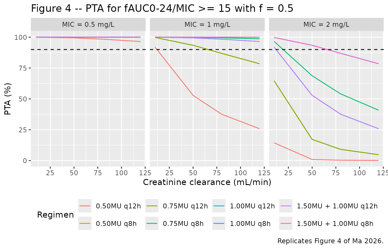
cell <- function(reg, mic, crcl) {
  v <- pta$PTA[pta$regimen == reg & pta$MIC == mic & pta$CRCL == crcl]
  if (length(v) != 1L) stop("no unique PTA cell for '", reg, "'")
  v
}

claims <- tibble::tribble(
  ~Claim, ~Source, ~Holds,
  "MIC = 0.5: all eight regimens exceed 90% PTA at every CrCl",
  "Results, Monte Carlo Simulation",
  all(pta$PTA[pta$MIC == 0.5] > 90),

  "MIC = 1.0: 0.50MU q12h reaches 90% only at CrCl <= 10 mL/min",
  "Results, Monte Carlo Simulation",
  cell("0.50MU q12h", 1, 10) > 90 &&
    all(vapply(c(50, 80, 120), function(k) cell("0.50MU q12h", 1, k) < 90,
               logical(1))),

  "MIC = 1.0: 0.50MU q8h and 0.75MU q12h fall below 90% at CrCl >= 80 mL/min",
  "Results, Monte Carlo Simulation",
  all(pta$PTA[pta$MIC == 1 & pta$CRCL >= 80 &
                pta$regimen %in% c("0.50MU q8h", "0.75MU q12h")] < 90),

  "MIC = 1.0: every other regimen exceeds 90% at every CrCl",
  "Results, Monte Carlo Simulation",
  all(pta$PTA[pta$MIC == 1 &
                !pta$regimen %in% c("0.50MU q12h", "0.50MU q8h",
                                    "0.75MU q12h")] > 90),

  "MIC = 2.0: no regimen reaches 90% at CrCl >= 80 mL/min",
  "Results and Conclusion",
  all(pta$PTA[pta$MIC == 2 & pta$CRCL >= 80] < 90)
)

knitr::kable(claims, caption = paste(
  "Every target-attainment claim Ma 2026 makes about Figure 4, checked",
  "against the packaged model."
))| Claim | Source | Holds |
|---|---|---|
| MIC = 0.5: all eight regimens exceed 90% PTA at every CrCl | Results, Monte Carlo Simulation | TRUE |
| MIC = 1.0: 0.50MU q12h reaches 90% only at CrCl <= 10 mL/min | Results, Monte Carlo Simulation | TRUE |
| MIC = 1.0: 0.50MU q8h and 0.75MU q12h fall below 90% at CrCl >= 80 mL/min | Results, Monte Carlo Simulation | TRUE |
| MIC = 1.0: every other regimen exceeds 90% at every CrCl | Results, Monte Carlo Simulation | TRUE |
| MIC = 2.0: no regimen reaches 90% at CrCl >= 80 mL/min | Results and Conclusion | TRUE |
# Deterministic: closed-form probabilities, not a simulated cohort.
stopifnot(nrow(claims) == 5L, all(claims$Holds))
All five published target-attainment conclusions – including the one that drives the paper’s clinical recommendation, that no regimen attains the target at MIC >= 2 mg/L in patients with preserved renal function – follow from the packaged model.
Assumptions and deviations
-
IIV scale. Table 3 heads the
inter-individual-variability row “Between-subject variability omega^2
CL”. The packaged model reads the tabulated 0.282 as a standard
deviation (
etalcl ~ 0.282^2), not a variance. This is not a preference: the dose-ratio probit identity applied to the paper’s own Table 4 returnsomega= 0.273, the variance reading misses all 64 Table 4 cells by an order of magnitude more than the packaged reading, and the digitised Figure 3 trough spread agrees with the packaged reading (95th/5th ratio near 12 against a digitised 8.7) and not with the variance one (which does not fall below 65). The tabulated RSE of 24.5% is the one piece of evidence pointing the other way – it is larger than the 9.9% one would expect for a standard deviation from 51 subjects and close to the 19.8% expected for a variance – and it is noted here as the reason the ambiguity is real rather than clerical. -
Residual-error scale. Table 3 heads the residual
row “Residual variability sigma^2” and gives 0.391, but the Results text
states that the EPS variance was fixed at 1 and that the
estimated quantity is the proportional coefficient
theta_prop. The packaged model therefore usespropSd = 0.391, a 39.1% proportional error. - Base-model table not used. Table 2 reports the base model with a residual of 1.19 against the final model’s 0.391. No single covariate on CL can reduce residual error by a factor of three, particularly given the reported dOFV of only -10.705, so Table 2’s residual row appears to be misreported. Nothing in the packaged model comes from Table 2; the base model is not extracted.
- CrCl centring constant. The value 94.76 mL/min appears only inside the final-model equation printed on p. 7. It is not tabulated, and it is not the cohort mean of 100.42 mL/min from Table 1. It is most consistent with the cohort median, which the paper does not report.
- IU-to-mg conversion is derived, not printed. The paper reports doses in international units and the model works in mg. The conversion of 43.8 mg per 10^6 IU used in the simulations above is recovered from Ma 2026’s own Table 4, cell by cell, with a coefficient of variation of 2.2% across cells. It is not needed to use the model – the model itself is in mg and mg/L – only to restate the paper’s IU regimens.
- Figure 3 percentiles are maintainer-digitised. The 5th, 50th and 95th observed percentile values at 1.5 h and 11.5 h after dose were read off the published Figure 3 panel by on-screen digitisation, to roughly +/- 0.05 mg/L. They appear nowhere in the text or tables. The Figure 3 comparison above is therefore indicative; the Table 4 reproduction, which uses printed numbers only, carries the weight.
-
Published AUC0-24,ss. The Discussion’s 12.83 +/-
7.57 mg*h/L is reproduced by the model only when read as a
free-drug exposure (
f = 0.5); as a total-drug exposure it is low by a factor of two and is inconsistent with the paper’s own observed concentration range. The comparison table above is against the number as printed, so it stars. - Body weight is not in the model. Table 1 reports BMI but not weight, and no size covariate was retained, so none is encoded. Weight enters only indirectly, through the Cockcroft-Gault CrCl the user supplies.
-
Sex was screened and dropped. Sex entered the full
regression model and was removed in backward elimination with no
reported coefficient. It is documented in
covariatesDataExcludedand is not encoded. - Creatinine-clearance distribution in the virtual cohort. The paper reports only the mean, SD and range. The cohort here draws from a gamma distribution matched to that mean and SD and truncated to the observed range; the true shape is unknown. None of the gated checks depends on this choice – the Table 4, Figure 4 and closed-form identity checks are all either at fixed creatinine clearance or per subject.
-
No PD or exposure-response model is extracted. The
fAUC/MIC >= 15target is quoted from Cheah et al, not fitted here, and the clinical- and microbiological-efficacy rates are descriptive. The paper contributes one model: the population PK model above. -
Steady state is imposed by repeated dosing, not by an
ssflag. Each simulated subject receives ten to fifteen doses before the observation window, which is far past steady state for a 4.2 h terminal half-life.