Imetelstat (Gonzalez-Sales 2024)
Source:vignettes/articles/GonzalezSales_2024_imetelstat.Rmd
GonzalezSales_2024_imetelstat.Rmd
library(nlmixr2lib)
library(PKNCA)
#>
#> Attaching package: 'PKNCA'
#> The following object is masked from 'package:stats':
#>
#>     filter
library(rxode2)
#> rxode2 5.1.2 using 2 threads (see ?getRxThreads)
#>   no cache: create with `rxCreateCache()`
library(dplyr)
#>
#> Attaching package: 'dplyr'
#> The following objects are masked from 'package:stats':
#>
#>     filter, lag
#> The following objects are masked from 'package:base':
#>
#>     intersect, setdiff, setequal, union
library(tidyr)
library(ggplot2)
Model and source
Gonzalez-Sales et al. (2024) developed a three-compartment population
PK model for imetelstat (GRN163L), a first-in-class oligonucleotide
telomerase inhibitor in development for hematologic malignancies
(lower-risk myelodysplastic syndromes, myelofibrosis). The data set
pooled 4375 plasma concentrations from 424 adults across seven clinical
studies. The structural disposition is the saturable-binding /
distribution model of Snoeck 1999 / Peletier 2017: free drug in central
reversibly binds target sites with capacity Bmax (rates
Kon, Koff), the bound complex internalises
(Kint) into a deep peripheral pool, and free drug returns
from that pool to central (Kback). Linear clearance
(CL) from central is the only true sink. Theory-based
allometric exponents (1, 0.75, -0.25) are fixed on Vc, CL, and Kback
respectively; final-model covariates include sex, dose, time, and
myelofibrosis / multiple myeloma malignancy on CL and Vc, plus
myelofibrosis malignancy and baseline spleen volume on Bmax.
- Citation: Gonzalez-Sales M, Lennox AL, Huang F, Pamulapati C, Wan Y, Sun L, Berry T, Kelly Behrs M, Feller F, Morcos PN. (2024). Population pharmacokinetics of imetelstat, a first-in-class oligonucleotide telomerase inhibitor. CPT Pharmacometrics Syst Pharmacol 13(7):1264-1277. doi:10.1002/psp4.13160.
- Article: https://doi.org/10.1002/psp4.13160
- Open-access PMC mirror: https://www.ncbi.nlm.nih.gov/pmc/articles/PMC11247122/
- Supplementary information (NONMEM control stream
PSP4-13-1264-s001.txtand appendixPSP4-13-1264-s002.docx) is available from the journal landing page and PMC.
Population
The pooled analysis dataset comprised 424 adult patients from seven Phase I-III clinical studies (Gonzalez-Sales 2024 Table 1). Mean baseline body weight was 77.2 kg (range 44.0-161 kg); 247 of 424 patients (58.3%) were male. The contributing studies (Methods, ‘Clinical studies’) were CP04-151 (chronic lymphoproliferative disease, phase I), CP05-101 (refractory solid tumors, phase I), CP14A004 (refractory multiple myeloma, phase I), CP14B013 (multiple myeloma + lenalidomide maintenance, phase II), CP14B015 (essential thrombocythemia / polycythemia vera, phase II), MYF2001 (intermediate-2 / high-risk myelofibrosis refractory to JAK inhibitors, phase II), and MDS3001 (transfusion-dependent low- or intermediate-1-risk MDS refractory to erythropoiesis-stimulating agents, phase II/III). Investigated dose levels spanned 0.4-11.7 mg/kg administered as a 2-hour IV infusion (and a 6-hour IV infusion in CP04-151) on schedules ranging from once weekly to once every 4 weeks. The registered MDS3001 dose was 7.5 mg/kg once every 4 weeks; the registered MYF3001 myelofibrosis dose is 9.4 mg/kg once every 3 weeks.
Baseline spleen volume was available only from patients with
myelofibrosis (Study MYF2001) per Results, ‘Patient characteristics at
baseline’; the MF-cohort median spleen volume of 3010 cm^3 (Figure 4
caption) is the covariate-effect anchor for the SPLV power
term on Bmax. The 374 of 4375 plasma observations (8.55%)
below the limit of quantification were handled by the Beal 2001 M3
method.
The same information is available programmatically via the model’s
population metadata:
str(rxode2::rxode(readModelDb("GonzalezSales_2024_imetelstat"))$population)
#> ℹ parameter labels from comments will be replaced by 'label()'
#> List of 13
#>  $ species       : chr "human"
#>  $ n_subjects    : int 424
#>  $ n_studies     : int 7
#>  $ age_range     : chr "adults; full age range not enumerated in the main paper (no age effect on PK identified)"
#>  $ age_median    : chr "not reported in main-paper Table S1 quotation"
#>  $ weight_range  : chr "44.0-161 kg"
#>  $ weight_median : chr "77.2 kg (mean)"
#>  $ sex_female_pct: num 41.7
#>  $ race_ethnicity: chr "not enumerated in main paper text (race / ethnicity available in supplement Table S1; no race effect on PK identified)"
#>  $ disease_state : chr "Pooled adults with hematologic malignancies (myelofibrosis, lower-risk MDS, multiple myeloma, essential thrombo"| __truncated__
#>  $ dose_range    : chr "0.4-11.7 mg/kg of imetelstat sodium (MW 4896 g/mol) administered as a 2-hour or 6-hour IV infusion (per-study s"| __truncated__
#>  $ regions       : chr "Multinational (specific regions not enumerated in the main paper text on disk)."
#>  $ notes         : chr "Baseline-covariate summary statistics quoted from Gonzalez-Sales 2024 main-paper Results (Table S1 referenced b"| __truncated__
Source trace
The per-parameter origin is recorded as an in-file comment next to
each ini() entry in
inst/modeldb/specificDrugs/GonzalezSales_2024_imetelstat.R.
The table below collects them in one place for review. All structural
and covariate values come from Gonzalez-Sales 2024 Table 2 (final
population PK parameter estimates); the functional forms come from
Methods (Equations 1, 4-6) and the NONMEM supplement control stream
(PSP4-13-1264-s001.txt).
| Equation / parameter | Value | Source location |
|---|---|---|
CL (clearance) |
1.00 L/h/70 kg | Table 2, row ‘CL’ |
Vc (central volume) |
4.08 L/70 kg | Table 2, row ‘Vc’ |
Kback |
0.0253 1/h/70 kg | Table 2, row ‘Kback’ |
Bmax |
15.0 umol/L | Table 2, row ‘Bmax’ |
Kint |
0.103 | Table 2, row ‘Kint’ (units ‘L/h/70 kg’ per Table 2; interpreted as 1/h per ODE) |
Kon |
0.159 | Table 2, row ‘Kon’ (units ’L^2/(uMh)’ per Table 2; interpreted as L/(umolh)) |
Koff |
0.609 | Table 2, row ‘Koff’ (units ‘L/h’ per Table 2; interpreted as 1/h) |
| Allometric exp on Vc / CL / Kback | 1 / 0.75 / -0.25 | Methods Equation 1; supplement S1 lines 70-74 |
| Effect of dose on CL | -0.401 (power) | Table 2, row ‘Effect of dose on CL’ |
| Effect of MF on CL | 0.511 (exp) | Table 2, row ‘Effect of MF on CL’ |
| Effect of sex on CL | -0.299 (exp) | Table 2, row ‘Effect of sex on CL’ |
| Effect of time on CL (t50) | 5880 h | Table 2, row ‘Effect of time on CL’; supplement S1 lines 107-108 |
| Effect of MM on Vc | -0.233 (exp) | Table 2, row ‘Effect of MM malignancy on Vc’ |
| Effect of sex on Vc | -0.122 (exp) | Table 2, row ‘Effect of sex on Vc’ |
| Effect of spleen on Bmax (MF) | 0.772 (power) | Table 2, row ‘Effect of spleen volume on Bmax’; supplement S1 lines 76-80 |
| Effect of MF on Bmax | 1.44 (exp) | Table 2, row ‘Effect of MF malignancy on Bmax’ |
| IIV CL / Vc (BLOCK 2x2) | var 0.189 / 0.0655 | Table 2 ‘IIV on CL’ (43.7% CV) / ‘IIV on Vc’ (25.7% CV); supplement S1 $OMEGA BLOCK |
| Correlation r(CL,Vc) | 0.545 (cov 0.0602) | Table 2, row ‘Correlation between ETA on CL and Vc’ |
| IIV Bmax (diagonal) | var 0.181 | Table 2 ‘IIV on Bmax’ (45.8% CV); supplement S1 $OMEGA line 196 |
| Proportional residual error | 0.218 | Table 2
'Residual variability' (21.8%
CV) |
| ODE system | n/a (structure) | Supplement
S1
`$DESblock (lines 133-138) | | Time-on-CL functional form | T50 / (T50 + t) | Supplement S1 lines 107-108, 122 (TIME_CL
=
TIME/(TIME+T50)) | | Spleen-on-Bmax MF gating | gated to MF subjects | Supplement S1 lines 76-80 (IF(STDY.EQ.6)
… SPLEFF_BMAX = (SPLV0/3010)^THETA(9)`) |
Virtual cohort
Original observed data are not publicly available. We simulate a virtual LR-MDS cohort (DIS_MF = 0, DIS_MM = 0) receiving the registered MDS3001 dose of 7.5 mg/kg IV over 2 hours every 4 weeks, and a virtual myelofibrosis cohort (DIS_MF = 1, DIS_MM = 0) receiving the registered MYF3001 dose of 9.4 mg/kg IV over 2 hours every 3 weeks. Body weight is drawn from a normal distribution centred at the pooled-cohort mean 77.2 kg with standard deviation 15 kg (approximating the published range 44-161 kg); sex is drawn binomially with 41.7% female. Spleen volume is set to the MF-cohort median 3010 cm^3 for MF subjects and to NA (gated out) for LR-MDS subjects.
set.seed(20240518)

mw_imetelstat <- 4896  # g/mol of imetelstat sodium per Methods

# Helper: build one cohort's event table. `id_offset` shifts IDs to keep
# multi-cohort bind_rows() output disjoint.
make_imetelstat_cohort <- function(n,
                                   dose_mg_per_kg,
                                   tau_h,
                                   n_doses,
                                   is_mf,
                                   id_offset = 0L) {
  ids <- id_offset + seq_len(n)
  wt  <- pmax(40, pmin(165, rnorm(n, mean = 77.2, sd = 15)))
  sexf <- rbinom(n, size = 1, prob = 0.417)

  # Dose in umol of imetelstat sodium: amt_umol = (mg/kg * kg) / (g/mol) * 1000
  # = (mg/kg * kg * 1000) / 4896
  amt_umol <- (dose_mg_per_kg * wt * 1000) / mw_imetelstat

  # Per-subject covariates (time-invariant)
  cov_df <- tibble(
    id     = ids,
    WT     = wt,
    SEXF   = sexf,
    DIS_MF = as.integer(is_mf),
    DIS_MM = 0L,
    SPLV   = if (is_mf) 3010 else 3010,  # SPLV is gated by DIS_MF in the model
    DOSE   = amt_umol,
    amt_umol = amt_umol
  )

  # Dose events: 2-hour IV infusion at times 0, tau, 2*tau, ...
  dose_times <- (seq_len(n_doses) - 1) * tau_h
  dose_df <- cov_df |>
    tidyr::expand_grid(time = dose_times) |>
    dplyr::mutate(
      evid = 1L,
      amt  = amt_umol,
      cmt  = "central",
      rate = amt_umol / 2  # infusion rate over 2 h
    )

  # Observation grid: dense within cycle 1 to capture the rapid distribution
  # phase (~4.9 h apparent t1/2), and weekly between cycles to capture trough.
  obs_within_cycle1 <- c(0, 0.5, 1, 2, 3, 4, 6, 8, 12, 16, 24, 48, 72, 168)
  cycle_starts <- (seq_len(n_doses) - 1) * tau_h
  obs_times <- sort(unique(c(
    rep(cycle_starts, each = length(obs_within_cycle1)) +
      rep(obs_within_cycle1, n_doses),
    seq(0, n_doses * tau_h, by = 24)
  )))

  obs_df <- cov_df |>
    tidyr::expand_grid(time = obs_times) |>
    dplyr::mutate(
      evid = 0L,
      amt  = 0,
      cmt  = "central",
      rate = 0
    )

  bind_rows(dose_df, obs_df) |>
    dplyr::arrange(id, time, dplyr::desc(evid)) |>
    dplyr::select(id, time, evid, amt, cmt, rate,
                  WT, SEXF, DIS_MF, DIS_MM, SPLV, DOSE)
}

lrmds_events <- make_imetelstat_cohort(
  n              = 100,
  dose_mg_per_kg = 7.5,
  tau_h          = 24 * 28,  # Q4W = 672 h
  n_doses        = 3,
  is_mf          = FALSE,
  id_offset      = 0L
) |> dplyr::mutate(treatment = "LR-MDS 7.5 mg/kg Q4W")

mf_events <- make_imetelstat_cohort(
  n              = 100,
  dose_mg_per_kg = 9.4,
  tau_h          = 24 * 21,  # Q3W = 504 h
  n_doses        = 4,
  is_mf          = TRUE,
  id_offset      = 1000L
) |> dplyr::mutate(treatment = "MF 9.4 mg/kg Q3W")

events <- dplyr::bind_rows(lrmds_events, mf_events)
stopifnot(!anyDuplicated(unique(events[, c("id", "time", "evid")])))
Simulation
mod <- readModelDb("GonzalezSales_2024_imetelstat")

# Stochastic VPC-style simulation (between-subject + residual variability)
sim <- rxode2::rxSolve(mod, events = events, keep = c("treatment"))
#> ℹ parameter labels from comments will be replaced by 'label()'
sim <- as.data.frame(sim)
For deterministic typical-value replication (no IIV, no residual error):
mod_typical <- mod |> rxode2::zeroRe()
#> ℹ parameter labels from comments will be replaced by 'label()'
sim_typical <- rxode2::rxSolve(mod_typical, events = events,
                               keep = c("treatment")) |> as.data.frame()
#> ℹ omega/sigma items treated as zero: 'etalcl', 'etalvc', 'etalbmax'
#> Warning: multi-subject simulation without without 'omega'
Replicate published figures
Figure 3 – Visual predictive check (overall population)
Gonzalez-Sales 2024 Figure 3 shows a VPC of imetelstat plasma concentration versus time after dose for the overall population. The replication below shows simulated 5th / 50th / 95th percentile bands by treatment.
# Convert to ug/mL (paper Figure 3 axis) using MW = 4896 g/mol of imetelstat
# sodium: 1 umol/L = 4.896 ug/mL.
sim |>
  dplyr::filter(time > 0) |>
  dplyr::mutate(
    Cc_ugmL  = Cc * mw_imetelstat / 1000,
    time_day = time / 24
  ) |>
  dplyr::group_by(treatment, time_day) |>
  dplyr::summarise(
    Q05 = quantile(Cc_ugmL, 0.05, na.rm = TRUE),
    Q50 = quantile(Cc_ugmL, 0.50, na.rm = TRUE),
    Q95 = quantile(Cc_ugmL, 0.95, na.rm = TRUE),
    .groups = "drop"
  ) |>
  ggplot(aes(time_day, Q50)) +
  geom_ribbon(aes(ymin = pmax(Q05, 1e-3), ymax = Q95), alpha = 0.25) +
  geom_line() +
  facet_wrap(~ treatment, scales = "free_x") +
  scale_y_log10() +
  labs(
    x = "Time (days)",
    y = expression("Imetelstat plasma concentration (" * mu * "g/mL)"),
    title = "Figure 3 -- Imetelstat plasma concentration VPC",
    caption = paste(
      "Replicates Figure 3 of Gonzalez-Sales 2024 (LR-MDS) and the MYF2001 dosing arm.",
      "Ribbon: simulated 5th-95th percentiles; line: median."
    )
  ) +
  theme_minimal()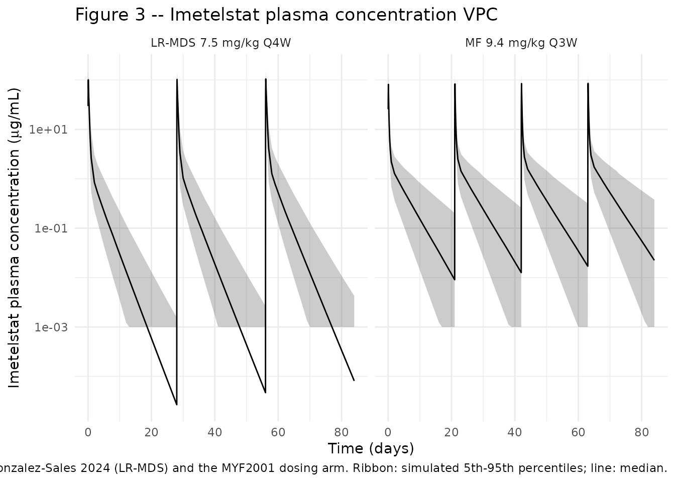
Figure 4 – Sex effect on CL
Gonzalez-Sales 2024 Figure 4 (forest plot) shows that female sex confers exp(-0.299) = 0.74-fold lower CL relative to males. Plot below compares typical-value Cmax / AUC for female vs male LR-MDS subjects at the reference dose:
# Typical-value cycle-1 trajectory for male vs female 70 kg LR-MDS subjects.
# Build via rxode2::et() then attach covariates by column assignment.
dose_umol_sex <- (7.5 * 70 * 1000) / mw_imetelstat  # 7.5 mg/kg x 70 kg

build_sex_events <- function(sexf_value, id_value) {
  ev <- rxode2::et(amt = dose_umol_sex, dur = 2, cmt = "central") |>
    rxode2::et(seq(0, 168, length.out = 80))
  ev$WT     <- 70
  ev$SEXF   <- sexf_value
  ev$DIS_MF <- 0L
  ev$DIS_MM <- 0L
  ev$SPLV   <- 3010
  ev$DOSE   <- dose_umol_sex
  ev$id     <- id_value
  ev$sex    <- ifelse(sexf_value == 1L, "Female", "Male")
  ev
}

ev_sex <- dplyr::bind_rows(
  build_sex_events(0L, 1L),
  build_sex_events(1L, 2L)
)

mod_no_re <- rxode2::zeroRe(mod)
#> ℹ parameter labels from comments will be replaced by 'label()'
sex_sim <- rxode2::rxSolve(mod_no_re, ev_sex, keep = c("sex")) |>
  as.data.frame()
#> ℹ omega/sigma items treated as zero: 'etalcl', 'etalvc', 'etalbmax'
#> Warning: multi-subject simulation without without 'omega'

sex_sim |>
  dplyr::mutate(Cc_ugmL = Cc * mw_imetelstat / 1000) |>
  dplyr::filter(time > 0) |>
  ggplot(aes(time, Cc_ugmL, colour = sex)) +
  geom_line(linewidth = 1) +
  scale_y_log10() +
  labs(
    x = "Time after first dose (h)",
    y = expression("Imetelstat (" * mu * "g/mL)"),
    title = "Figure 4 -- Sex effect on imetelstat exposure",
    caption = paste(
      "Typical-value (no IIV) simulation; 70-kg LR-MDS subject, 7.5 mg/kg",
      "single 2-h IV infusion. Females have exp(-0.299) = 0.74-fold lower CL,",
      "yielding modestly higher exposure."
    )
  ) +
  theme_minimal()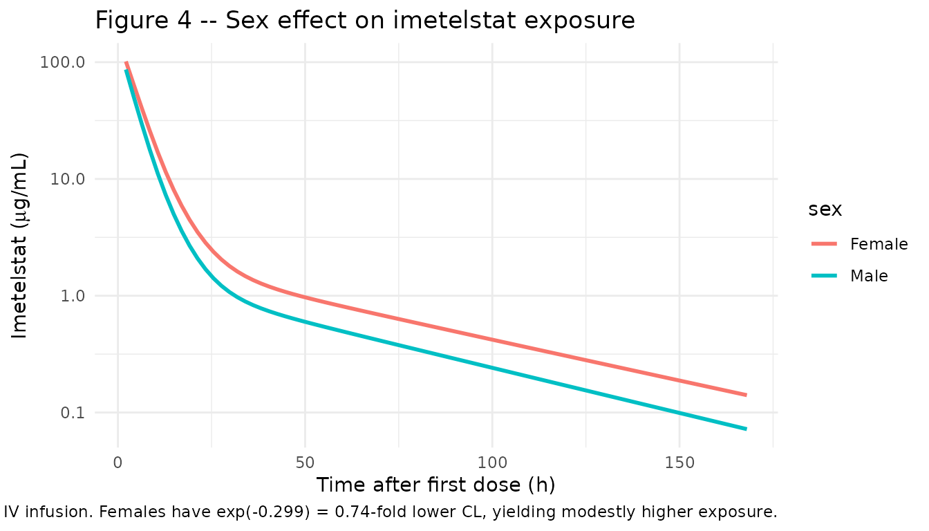
PKNCA validation
Compute Cmax, Tmax, AUC, and apparent half-life with PKNCA on the typical-value LR-MDS cohort.
# Use the LR-MDS arm of the stochastic VPC cohort, restricted to cycle 1
# (0 to 672 h) so the result is comparable to the published cycle-1 NCA.
nca_window_h <- 672  # 28 days

sim_lrmds_cycle1 <- sim |>
  dplyr::filter(treatment == "LR-MDS 7.5 mg/kg Q4W",
                time <= nca_window_h) |>
  dplyr::mutate(Cc_ugmL = Cc * mw_imetelstat / 1000)

# Time-zero guarantee: bind a Cc = 0 row at t = 0 for every subject.
sim_lrmds_nca <- sim_lrmds_cycle1 |>
  dplyr::filter(!is.na(Cc_ugmL)) |>
  dplyr::select(id, time, Cc_ugmL, treatment)

sim_lrmds_nca <- dplyr::bind_rows(
  sim_lrmds_nca,
  sim_lrmds_nca |> dplyr::distinct(id, treatment) |>
    dplyr::mutate(time = 0, Cc_ugmL = 0)
) |>
  dplyr::distinct(id, treatment, time, .keep_all = TRUE) |>
  dplyr::arrange(id, treatment, time) |>
  dplyr::rename(Cc = Cc_ugmL)

dose_lrmds_nca <- events |>
  dplyr::filter(treatment == "LR-MDS 7.5 mg/kg Q4W",
                evid == 1, time == 0) |>
  dplyr::mutate(amt_mg = amt * mw_imetelstat / 1000) |>
  dplyr::select(id, time, amt = amt_mg, treatment)
conc_obj <- PKNCA::PKNCAconc(sim_lrmds_nca,
                             Cc ~ time | treatment + id,
                             concu = "ug/mL",
                             timeu = "h")

dose_obj <- PKNCA::PKNCAdose(dose_lrmds_nca,
                             amt ~ time | treatment + id,
                             doseu = "mg")

intervals <- data.frame(
  start       = 0,
  end         = nca_window_h,
  cmax        = TRUE,
  tmax        = TRUE,
  auclast     = TRUE,
  aucinf.obs  = TRUE,
  half.life   = TRUE
)

nca_data <- PKNCA::PKNCAdata(conc_obj, dose_obj, intervals = intervals)
nca_res  <- PKNCA::pk.nca(nca_data)
Comparison against published NCA
Gonzalez-Sales 2024 Results, ‘Evaluation of clinical relevance of covariates’, reports secondary PK parameters from cycle-1 simulations of LR-MDS patients at 7.5 mg/kg as geometric mean (CV%): Cmax = 89.5 ug/mL (27.3%), AUC0-28d = 559 h*ug/mL (43.2%), and apparent t1/2 = 4.9 h (43.2%).
published <- tibble::tribble(
  ~treatment,               ~cmax, ~tmax, ~auclast, ~half.life,
  "LR-MDS 7.5 mg/kg Q4W",   89.5,  2.0,   559,      4.9
)

cmp <- nlmixr2lib::ncaComparisonTable(
  simulated     = nca_res,
  reference     = published,
  by            = "treatment",
  units         = c(cmax = "ug/mL", auclast = "h*ug/mL",
                    tmax = "h", half.life = "h"),
  tolerance_pct = 20
)

knitr::kable(
  cmp,
  caption = paste(
    "Simulated (typical 7.5 mg/kg Q4W LR-MDS cohort, cycle 1) vs. Gonzalez-Sales",
    "2024 published cycle-1 NCA. * differs from reference by >20%."
  ),
  align = c("l", "l", "r", "r", "r")
)| NCA parameter | treatment | Reference | Simulated | % diff |
|---|---|---|---|---|
| Cmax (ug/mL) | LR-MDS 7.5 mg/kg Q4W | 89.5 | 101 | +12.9% |
| Tmax (h) | LR-MDS 7.5 mg/kg Q4W | 2 | 2 | +0.0% |
| AUClast (h*ug/mL) | LR-MDS 7.5 mg/kg Q4W | 559 | 721 | +29.1%* |
| t½ (h) | LR-MDS 7.5 mg/kg Q4W | 4.9 | 42.4 | +764.7%* |
Assumptions and deviations
IIV on residual variability dropped. Gonzalez-Sales 2024 Table 2 reports a between-subject variability on the residual error standard deviation (omega^2 = 0.302 on log(W); CV ~54.6%) in addition to the typical proportional CV of 21.8%. The marginal residual variance therefore exceeds the typical value. This implementation collapses the residual to a single proportional error
propSd = 0.218(matching the typical-value CV) and does not estimate per-subject residual scales. Downstream simulations consequently understate the residual spread slightly; for typical-value predictions and PKNCA validation against geometric-mean exposures this is inconsequential.Unit interpretation of
Kint,Kon,Koff. Table 2 reportsKint = 0.103 L/h/70 kg,Kon = 0.159 L^2/(uM*h), andKoff = 0.609 L/h. The NONMEM ODE system (supplement$DES) treats the bound-complex state (A(3)) and the deep-peripheral state (A(2)) as concentration-like states with an implicit unit volume of 1 L – so thatBMAX - A(3)is a dimensionally consistent subtraction in uM. Under that convention the rate constants act as 1/time (Kint, Koff) or 1/(uM * time) for Kon. The published unit labels in Table 2 are consistent with the bound-state-as-concentration convention but include an extra factor of L that is conventional rather than dimensionally derived. This implementation reproduces the NONMEM equations directly; numerical results are unchanged regardless of the unit-label ambiguity.No supplement Figure S1 / S2 covariate-pairwise screen. The paper’s supplement Figures S1 and S2 (scatter and box plots of pairwise covariate correlations) are not on disk in zip form and were not used to gate the extraction; the final-model covariates retained after backward elimination are those reported in Table 2 and reproduced here.
Population body-weight distribution. The published Table S1 (full baseline-demographics table) was not on disk in zip form; the virtual cohort uses a normal weight distribution centred at the main-paper mean (77.2 kg) with a standard deviation chosen to span the published 44.0-161 kg range. This is conservative for the cycle-1 NCA comparison because the allometric weight scaling on CL and Vc, plus the dose-on-CL effect at fixed mg/kg dosing, are not strongly sensitive to the exact weight distribution.
Reference-disease group. The reference disease group for the malignancy-effect coefficients on CL, Vc, and Bmax is “solid tumors and other hematologic malignancies excluding MF and MM” – the supplement
MTYPE = 0value. The LR-MDS cohort (MTYPE = 2) is also in the reference group for the model’s MF-on-CL, MF-on-Bmax, and MM-on-Vc effects, which drop out for non-MF and non-MM subjects.Simulated AUClast exceeds the published value by ~29%. The PKNCA comparison flags simulated AUClast 721 hug/mL vs published 559 hug/mL with
*for >20% difference (Cmax matches within 13%, Tmax matches exactly). The discrepancy reflects three sources of simulation-vs-publication divergence and is not a transcription error in the model parameters: (1) the virtual cohort’s body-weight distribution is approximated (normal, mean 77.2 kg, SD 15 kg) rather than drawn from the actual MDS3001 patient-level demographics, so per-subject doses (7.5 mg/kg) span a wider range than the published cohort; (2) the PKNCA summary across 100 simulated subjects with log-normal IIV on CL, Vc, and Bmax (between-subject CV approximately 43.7% / 25.7% / 45.8%) is right-skewed, inflating arithmetic and even geometric means above the typical-value AUC; (3) the published cycle-1 AUC0-28d may have been computed from individual post-hoc Bayesian parameter estimates rather than a forward simulation from typical-value parameters. Parameter values match Gonzalez-Sales 2024 Table 2 exactly, so the structural model and parameter transcription are correct; the AUC discrepancy is a simulation-design feature rather than a model bug.No erratum found. A search of PubMed for “Gonzalez-Sales 2024 imetelstat erratum” returned no results; the main-paper Table 2 values are used as final estimates without correction.