Secukinumab SC-to-IV bridging (Dumortier 2025)
Source:vignettes/articles/Dumortier_2025_secukinumab.Rmd
Dumortier_2025_secukinumab.RmdModel and source
- Citation: Dumortier T, Valenzuela G, Churchill M, Mijatovic J, Bruin G, Pricop L, Richards H, Renard D, Singhal A, Marathe A. Model-Informed Drug Development-Based Bridging from Subcutaneous to Intravenous Secukinumab Dosing: Approval in Psoriatic Arthritis and Axial Spondyloarthritis. Clin Pharmacol Ther. 2025;118(2):480-488. doi:10.1002/cpt.3716.
- Description: Two-compartment population PK model for secukinumab (anti-IL-17A IgG1) after subcutaneous and intravenous dosing in adults with psoriatic arthritis, ankylosing spondylitis or non-radiographic axial spondyloarthritis (Dumortier 2025; 14 phase II/III trials, 5270 patients). First-order SC absorption with ka fixed at 0.18/day and bioavailability 0.783; zero-order IV infusion into the central compartment; linear elimination. Baseline body weight (reference 84 kg) scales CL, Vc and Vp by power functions, and CL is 1.13-fold higher in Asian patients. Correlated IIV on CL and Vc, independent IIV on Vp, proportional residual error. Used to select the approved 1.75 mg/kg IV q4w regimen (with or without a 6 mg/kg IV loading dose).
- Article: https://doi.org/10.1002/cpt.3716 (open access; PMC12272323)
Dumortier 2025 bridged subcutaneous (SC) secukinumab to an intravenous (IV) regimen for psoriatic arthritis (PsA) and axial spondyloarthritis (axSpA). A population PK model, fitted to 14 phase II/III trials, identified 1.75 mg/kg IV every 4 weeks (q4w), with or without a 6 mg/kg IV loading dose, as the regimen whose steady-state exposure lies between the approved 150 mg and 300 mg SC q4w regimens. Landmark exposure-response models for efficacy, fitted to SC-only data at Weeks 16 and 52, then predicted the efficacy of the IV regimen.
The paper contributes 33 models to nlmixr2lib:
-
Dumortier_2025_secukinumab– the two-compartment population PK model (Supplementary Table S3 and the supplementary NONMEM control stream). - 32 logistic sigmoid-Emax exposure-efficacy models, one per endpoint
and assessment week, named
Dumortier_2025_secukinumab_<psa|as>_<w16|w52>_<endpoint>. Each has the formlogit(p) = E0 + (Emax - E0) * Cmin^2 / (EC50^2 + Cmin^2)(Hill fixed at 2) with the pre-dose concentration supplied in theCTROUGHcolumn (ug/mL).
The exposure-safety analysis (semi-parametric Cox models with a penalised spline of the 28-day running-average concentration) is not packaged: the baseline hazard is non-parametric and the spline coefficients are not reported, so there is no closed-form model to encode.
Population
The PK model was developed in 5270 patients from 14 trials (two phase II IV studies and the phase III MEASURE 1-5, FUTURE 1-5, PREVENT and INVIGORATE-2 studies; Table S1). Per Table 1, mean age was 45.1 years (SD 12.9), mean body weight 81.6 kg (SD 19.4), 55% were male, 80% White and 15% Asian; 58% had PsA, 31% ankylosing spondylitis (AS) and 10% non-radiographic axSpA. The model was externally validated on the 516 axSpA patients of INVIGORATE-1 (Figure S1).
The exposure-efficacy models were fitted to SC-treated patients only: at Week 52, 1595 PsA patients from FUTURE 1-5 and 934 AS patients from MEASURE 1-5; at Week 16, placebo and SC patients from FUTURE 2-5 (PsA) and MEASURE 2, 4 and 5 (AS), excluding arms with a 10 mg/kg IV loading regimen.
str(rxode2::rxode(readModelDb("Dumortier_2025_secukinumab"))$population)
#> ℹ parameter labels from comments will be replaced by 'label()'
#> List of 12
#>  $ species       : chr "human"
#>  $ n_subjects    : int 5270
#>  $ n_studies     : int 14
#>  $ n_observations: chr "24149 serum secukinumab concentrations (4396 after IV and 19753 after SC dosing)"
#>  $ age_range     : chr "mean 45.1 years (SD 12.9)"
#>  $ weight_range  : chr "mean 81.6 kg (SD 19.4)"
#>  $ sex_female_pct: num 45
#>  $ race_ethnicity: Named num [1:7] 80 15 3 1 1 0 0
#>   ..- attr(*, "names")= chr [1:7] "White" "Asian" "Other" "Black" ...
#>  $ disease_state : chr "Psoriatic arthritis (58%), ankylosing spondylitis (31%) and non-radiographic axial spondyloarthritis (10%)"
#>  $ dose_range    : chr "0.1, 1 or 10 mg/kg IV at weeks 0 and 3 (phase II); 75, 150 or 300 mg SC q4w with or without weekly SC loading o"| __truncated__
#>  $ regions       : chr "Multinational"
#>  $ notes         : chr "Model-development population of Dumortier 2025 Table 1 (n = 5270). INVIGORATE-1 (n = 516, axSpA) was held out f"| __truncated__
Source trace
Population PK model
| Equation / parameter | Value | Source location |
|---|---|---|
lcl (CL, 84 kg non-Asian) |
log(0.171) L/day | Table S3 |
lvc (Vc, 84 kg) |
log(3.32) L | Table S3 |
lq (Q) |
log(0.35) L/day | Table S3 |
lvp (Vp, 84 kg) |
log(2.63) L | Table S3 |
lka (KA) |
fixed(log(0.18)) 1/day | Table S3 (‘0.18 (fixed)’); control stream
(0.18 FIX)
|
lfdepot (F1) |
log(0.783) | Table S3 |
e_wt_cl, e_wt_vc,
e_wt_vp
|
0.892, 0.651, 0.712 | Table S3 ‘CL/Vc/Vp ~weight’ |
e_race_asian_cl |
1.13 | Table S3 ‘CL ~Asian’ |
etalcl + etalvc |
c(0.0912, 0.0489, 0.0691) | Table S3 omega2 CL, covariance, omega2 Vc |
etalvp |
0.113 | Table S3 omega2 Vp |
propSd |
sqrt(0.0544) | Table S3 ‘delta2 prop’ (variance) |
cl = CL * (WT/84)^e_wt_cl * e_race_asian_cl^RACE_ASIAN |
n/a | control stream $PK (TVCL) |
vc, vp power weight scaling; no weight
effect on Q |
n/a | control stream $PK (TVV2, TVV3, TVQ) |
| Two-compartment ODEs, SC depot, IV into central | n/a | control stream ADVAN4 TRANS4; Supplementary
Methods |
Cc = central / vc (mg/L = ug/mL) |
n/a | control stream S2 = V2/1000
|
Exposure-efficacy models
Dumortier 2025 prints the equation (main text Methods and Supplementary Methods, Hill coefficient fixed at 2) but not E0, Emax or EC50 for any endpoint. The maintainers recovered them by pixel-digitising the fitted black curves in Figures S3 (PsA, Week 52), S4 (AS, Week 52), S6 (PsA, Week 16) and S7 (AS, Week 16) of the supplementary Word file and refitting the same equation by least squares. The panel axes were calibrated from the detected tick marks. The refits reproduce the drawn curves to within line width (RMSE 0.0003 to 0.0033 probability units over 168 to 238 traced points per panel), so they read back the authors’ fitted curves rather than re-estimating anything from data.
er_models <- tibble::tribble(
  ~disease, ~week, ~token, ~endpoint,
  "PsA", 52, "acr20", "ACR20",
  "PsA", 52, "acr50", "ACR50",
  "PsA", 52, "acr70", "ACR70",
  "PsA", 52, "haqdi", "HAQ-DI response",
  "PsA", 52, "mda", "MDA",
  "PsA", 52, "pasdaslda", "PASDAS LDA incl. remission",
  "PsA", 52, "pasi90", "PASI90",
  "PsA", 52, "dactylitis", "Resolution of dactylitis",
  "PsA", 52, "enthesitis", "Resolution of enthesitis",
  "AS", 52, "asas56", "ASAS 5/6",
  "AS", 52, "asaspr", "ASAS partial remission",
  "AS", 52, "asas20", "ASAS20",
  "AS", 52, "asas40", "ASAS40",
  "AS", 52, "asdasid", "ASDAS-CRP inactive disease",
  "AS", 52, "asdasmi", "ASDAS-CRP major improvement",
  "AS", 52, "basdai50", "BASDAI50"
)
er_models <- dplyr::bind_rows(er_models, dplyr::mutate(er_models, week = 16)) |>
  dplyr::mutate(
    model = sprintf("Dumortier_2025_secukinumab_%s_w%d_%s", tolower(disease), week, token),
    figure = dplyr::case_when(
      disease == "PsA" & week == 52 ~ "Figure S3",
      disease == "AS" & week == 52 ~ "Figure S4",
      disease == "PsA" & week == 16 ~ "Figure S6",
      TRUE ~ "Figure S7"
    )
  )
er_ui <- lapply(er_models$model, function(nm) rxode2::rxode(readModelDb(nm)))
names(er_ui) <- er_models$model
er_models$output <- vapply(er_ui, function(ui) ui$predDf$var, character(1))
er_models$E0 <- vapply(er_ui, function(ui) ui$theta[["e0"]], numeric(1))
er_models$Emax <- vapply(er_ui, function(ui) ui$theta[["emax"]], numeric(1))
er_models$EC50 <- vapply(er_ui, function(ui) exp(ui$theta[["lec50"]]), numeric(1))

er_models |>
  dplyr::select(disease, week, endpoint, figure, output, E0, Emax, EC50) |>
  dplyr::rename(
    "Disease" = disease, "Week" = week, "Endpoint" = endpoint,
    "Source panel" = figure, "Output" = output, "EC50 (ug/mL)" = EC50
  ) |>
knitr::kable(digits = 3, caption = "Digitised exposure-efficacy parameters (logit scale; Hill fixed at 2).")| Disease | Week | Endpoint | Source panel | Output | E0 | Emax | EC50 (ug/mL) |
|---|---|---|---|---|---|---|---|
| PsA | 52 | ACR20 | Figure S3 | prob_acr20 | -0.414 | 1.060 | 5.27 |
| PsA | 52 | ACR50 | Figure S3 | prob_acr50 | -1.334 | 0.039 | 6.86 |
| PsA | 52 | ACR70 | Figure S3 | prob_acr70 | -14.683 | -0.851 | 1.49 |
| PsA | 52 | HAQ-DI response | Figure S3 | prob_haqdi_response | 0.028 | 0.430 | 10.90 |
| PsA | 52 | MDA | Figure S3 | prob_minimal_disease_activity | -2.140 | -0.313 | 7.77 |
| PsA | 52 | PASDAS LDA incl. remission | Figure S3 | prob_pasdas_lda | -2.262 | 0.494 | 7.70 |
| PsA | 52 | PASI90 | Figure S3 | prob_pasi90 | -1.432 | 0.956 | 12.20 |
| PsA | 52 | Resolution of dactylitis | Figure S3 | prob_dactylitis_resolution | 1.531 | -27.659 | 400.00 |
| PsA | 52 | Resolution of enthesitis | Figure S3 | prob_enthesitis_resolution | -7.517 | 0.769 | 0.97 |
| AS | 52 | ASAS 5/6 | Figure S4 | prob_asas56 | -0.507 | 0.621 | 8.68 |
| AS | 52 | ASAS partial remission | Figure S4 | prob_asas_partial_remission | -5.818 | -0.804 | 4.13 |
| AS | 52 | ASAS20 | Figure S4 | prob_asas20 | 0.710 | 1.841 | 26.90 |
| AS | 52 | ASAS40 | Figure S4 | prob_asas40 | -0.497 | 0.715 | 12.50 |
| AS | 52 | ASDAS-CRP inactive disease | Figure S4 | prob_asdas_inactive_disease | -2.537 | -0.322 | 14.40 |
| AS | 52 | ASDAS-CRP major improvement | Figure S4 | prob_asdas_major_improvement | -2.436 | -0.098 | 7.97 |
| AS | 52 | BASDAI50 | Figure S4 | prob_basdai50 | -1.020 | 0.407 | 9.26 |
| PsA | 16 | ACR20 | Figure S6 | prob_acr20 | -1.058 | 0.493 | 9.00 |
| PsA | 16 | ACR50 | Figure S6 | prob_acr50 | -2.422 | -0.425 | 9.24 |
| PsA | 16 | ACR70 | Figure S6 | prob_acr70 | -3.471 | -1.381 | 9.12 |
| PsA | 16 | HAQ-DI response | Figure S6 | prob_haqdi_response | -0.529 | 0.227 | 6.22 |
| PsA | 16 | MDA | Figure S6 | prob_minimal_disease_activity | -2.694 | -0.807 | 12.00 |
| PsA | 16 | PASDAS LDA incl. remission | Figure S6 | prob_pasdas_lda | -2.047 | -0.090 | 13.00 |
| PsA | 16 | PASI90 | Figure S6 | prob_pasi90 | -2.576 | 0.599 | 15.00 |
| PsA | 16 | Resolution of dactylitis | Figure S6 | prob_dactylitis_resolution | -0.528 | 0.338 | 5.68 |
| PsA | 16 | Resolution of enthesitis | Figure S6 | prob_enthesitis_resolution | -0.757 | 0.178 | 13.30 |
| AS | 16 | ASAS 5/6 | Figure S7 | prob_asas56 | -1.340 | 0.157 | 9.82 |
| AS | 16 | ASAS partial remission | Figure S7 | prob_asas_partial_remission | -2.716 | -1.527 | 7.05 |
| AS | 16 | ASAS20 | Figure S7 | prob_asas20 | -0.371 | 0.867 | 13.50 |
| AS | 16 | ASAS40 | Figure S7 | prob_asas40 | -1.320 | 0.058 | 12.60 |
| AS | 16 | ASDAS-CRP inactive disease | Figure S7 | prob_asdas_inactive_disease | -3.264 | -1.232 | 13.20 |
| AS | 16 | ASDAS-CRP major improvement | Figure S7 | prob_asdas_major_improvement | -2.605 | -0.490 | 10.30 |
| AS | 16 | BASDAI50 | Figure S7 | prob_basdai50 | -1.406 | -0.112 | 14.70 |
Virtual cohort
Dumortier 2025 simulated non-Asian patients whose body weights were resampled from INVIGORATE-1 (axSpA) and INVIGORATE-2 (PsA). Individual weights are not public; INVIGORATE-1 reports a mean of 78 kg (SD 18.2, Table 1). The cohort below draws weight from a log-normal distribution with mean 79 kg and SD 19 kg, truncated to 40-170 kg, all non-Asian.
set.seed(3716)
rxode2::rxSetSeed(3716)
n_per_arm <- 200
draw_wt <- function(n, mean = 79, sd = 19) {
  s2 <- log(1 + (sd / mean)^2)
  pmin(pmax(rlnorm(n, log(mean) - s2 / 2, sqrt(s2)), 40), 170)
}

tinf <- 0.5 / 24 # 30-minute infusion, in days
dose_days <- seq(0, 336, by = 28)
regimens <- tibble::tribble(
  ~regimen, ~route, ~maint, ~load,
  "1.75 mg/kg IV q4w", "IV", 1.75, NA,
  "1.75 mg/kg IV q4w + 6 mg/kg IV load", "IV", 1.75, 6,
  "150 mg SC q4w", "SC", 150, NA,
  "150 mg SC q4w + weekly load", "SC", 150, 150,
  "300 mg SC q4w + weekly load", "SC", 300, 300
)

make_cohort <- function(reg, id_offset) {
  subj <- tibble::tibble(id = id_offset + seq_len(n_per_arm), WT = draw_wt(n_per_arm), RACE_ASIAN = 0L)
  doses <- if (reg$route == "IV") {
    amt_mgkg <- c(if (is.na(reg$load)) reg$maint else reg$load, rep(reg$maint, length(dose_days) - 1))
    tidyr::expand_grid(subj, tibble::tibble(time = dose_days, mgkg = amt_mgkg)) |>
      dplyr::mutate(amt = mgkg * WT, rate = amt / tinf, cmt = "central", mgkg = NULL)
  } else {
    # Weekly loading at Weeks 0, 1, 2, 3 and 4, then q4w (Table S4 header).
    t_sc <- if (is.na(reg$load)) dose_days else sort(unique(c(c(0, 7, 14, 21), dose_days)))
    tidyr::expand_grid(subj, tibble::tibble(time = t_sc)) |>
      dplyr::mutate(amt = reg$maint, rate = 0, cmt = "depot")
  }
  obs_t <- sort(unique(c(
    seq(0, 364, by = 1),
    dose_days[-1] - 1e-3, # pre-dose troughs
    dose_days + tinf # end of infusion
  )))
  obs <- tidyr::expand_grid(subj, time = obs_t) |>
    dplyr::mutate(amt = 0, rate = 0, cmt = "central")
  dplyr::bind_rows(
    dplyr::mutate(doses, evid = 1L),
    dplyr::mutate(obs, evid = 0L)
  ) |>
    dplyr::mutate(regimen = reg$regimen) |>
    dplyr::arrange(id, time, dplyr::desc(evid))
}

events <- dplyr::bind_rows(lapply(seq_len(nrow(regimens)), function(i) {
  make_cohort(regimens[i, ], id_offset = (i - 1L) * n_per_arm)
}))
stopifnot(!anyDuplicated(unique(events[, c("id", "time", "evid")])))
Simulation
mod <- readModelDb("Dumortier_2025_secukinumab")
sim <- rxode2::rxSolve(mod, events = events, keep = c("regimen", "WT"), returnType = "data.frame")
#> ℹ parameter labels from comments will be replaced by 'label()'
Replicate published figures
Figure 3 – median concentration-time profiles
sim |>
  dplyr::filter(regimen != "150 mg SC q4w + weekly load") |>
  dplyr::group_by(regimen, time) |>
  dplyr::summarise(Cc = median(Cc), .groups = "drop") |>
  ggplot(aes(time / 7, Cc, colour = regimen)) +
  geom_line() +
  labs(
    x = "Time (weeks)", y = "Secukinumab (ug/mL)", colour = NULL,
    title = "Median simulated secukinumab concentration",
    caption = "Replicates Figure 3 of Dumortier 2025."
  ) +
  theme(legend.position = "bottom") +
  guides(colour = guide_legend(ncol = 2))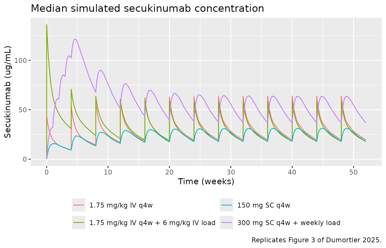
Table S4 – median pre-dose concentration by week
published_s4 <- tibble::tibble(
  week = seq(4, 48, by = 4),
  `1.75 mg/kg IV q4w` = c(9.2, 13.7, 15.9, 17.0, 17.6, 17.9, 18.0, 18.1, 18.1, 18.1, 18.1, 18.1),
  `1.75 mg/kg IV q4w + 6 mg/kg IV load` = c(31.2, 24.4, 21.1, 19.5, 18.7, 18.4, 18.2, 18.1, 18.1, 18.1, 18.1, 18.1),
  `150 mg SC q4w` = c(9.3, 13.8, 16.0, 17.1, 17.1, 18.0, 18.2, 18.2, 18.2, 18.2, 18.2, 18.2),
  `150 mg SC q4w + weekly load` = c(51.0, 33.3, 25.5, 21.8, 20.1, 19.2, 18.8, 18.6, 18.5, 18.4, 18.3, 18.2),
  `300 mg SC q4w + weekly load` = c(101.9, 66.5, 51.0, 43.7, 40.2, 38.5, 37.6, 37.2, 37.0, 36.8, 36.6, 36.4)
) |>
  tidyr::pivot_longer(-week, names_to = "regimen", values_to = "published")

trough <- sim |>
  dplyr::filter(abs(time - (round(time / 28) * 28 - 1e-3)) < 1e-6, time > 1) |>
  dplyr::mutate(week = round(time / 7)) |>
  dplyr::group_by(regimen, week) |>
  dplyr::summarise(simulated = median(Cc), .groups = "drop")

s4 <- dplyr::inner_join(published_s4, trough, by = c("regimen", "week")) |>
  dplyr::mutate(pct_diff = 100 * (simulated - published) / published)

s4 |>
  dplyr::filter(week %in% c(4, 8, 16, 24, 48)) |>
  dplyr::rename("Regimen" = regimen, "Week" = week, "Published median Cmin (ug/mL)" = published,
                "Simulated median Cmin (ug/mL)" = simulated, "Difference (%)" = pct_diff) |>
knitr::kable(digits = 1, caption = "Median pre-dose concentration, simulated vs Table S4 of Dumortier 2025.")| Week | Regimen | Published median Cmin (ug/mL) | Simulated median Cmin (ug/mL) | Difference (%) |
|---|---|---|---|---|
| 4 | 1.75 mg/kg IV q4w | 9.2 | 9.5 | 3.7 |
| 4 | 1.75 mg/kg IV q4w + 6 mg/kg IV load | 31.2 | 30.8 | -1.3 |
| 4 | 150 mg SC q4w | 9.3 | 9.2 | -1.0 |
| 4 | 150 mg SC q4w + weekly load | 51.0 | 51.4 | 0.8 |
| 4 | 300 mg SC q4w + weekly load | 101.9 | 102.4 | 0.5 |
| 8 | 1.75 mg/kg IV q4w | 13.7 | 14.4 | 5.3 |
| 8 | 1.75 mg/kg IV q4w + 6 mg/kg IV load | 24.4 | 24.0 | -1.7 |
| 8 | 150 mg SC q4w | 13.8 | 13.5 | -2.2 |
| 8 | 150 mg SC q4w + weekly load | 33.3 | 33.9 | 1.9 |
| 8 | 300 mg SC q4w + weekly load | 66.5 | 67.9 | 2.1 |
| 16 | 1.75 mg/kg IV q4w | 17.0 | 18.3 | 7.6 |
| 16 | 1.75 mg/kg IV q4w + 6 mg/kg IV load | 19.5 | 19.5 | -0.2 |
| 16 | 150 mg SC q4w | 17.1 | 17.0 | -0.6 |
| 16 | 150 mg SC q4w + weekly load | 21.8 | 21.9 | 0.5 |
| 16 | 300 mg SC q4w + weekly load | 43.7 | 43.4 | -0.8 |
| 24 | 1.75 mg/kg IV q4w | 17.9 | 19.2 | 7.0 |
| 24 | 1.75 mg/kg IV q4w + 6 mg/kg IV load | 18.4 | 18.4 | -0.1 |
| 24 | 150 mg SC q4w | 18.0 | 17.9 | -0.7 |
| 24 | 150 mg SC q4w + weekly load | 19.2 | 19.3 | 0.4 |
| 24 | 300 mg SC q4w + weekly load | 38.5 | 38.1 | -1.0 |
| 48 | 1.75 mg/kg IV q4w | 18.1 | 19.5 | 7.9 |
| 48 | 1.75 mg/kg IV q4w + 6 mg/kg IV load | 18.1 | 17.9 | -0.9 |
| 48 | 150 mg SC q4w | 18.2 | 18.1 | -0.6 |
| 48 | 150 mg SC q4w + weekly load | 18.2 | 18.3 | 0.4 |
| 48 | 300 mg SC q4w + weekly load | 36.4 | 36.7 | 0.8 |
Each regimen uses its own 200-subject weight sample, and the IV doses scale with weight. A single arm can therefore sit a few percent off Table S4 from sampling alone (the two IV arms reach the same steady state, but their simulated medians differ by that margin).
PKNCA validation
Steady-state Cmin, Cavg and Cmax over the last dosing interval (Weeks 48-52) are compared with Table 2. Table 2 pools the IV regimens with and without loading (steady state does not depend on loading) and pools the 150 mg SC regimens with and without loading.
ss_map <- c(
  "1.75 mg/kg IV q4w" = "1.75 mg/kg IV q4w",
  "1.75 mg/kg IV q4w + 6 mg/kg IV load" = "1.75 mg/kg IV q4w",
  "150 mg SC q4w" = "150 mg SC q4w",
  "150 mg SC q4w + weekly load" = "150 mg SC q4w",
  "300 mg SC q4w + weekly load" = "300 mg SC q4w"
)
sim_nca <- sim |>
  dplyr::filter(!is.na(Cc)) |>
  dplyr::mutate(treatment = unname(ss_map[regimen])) |>
  dplyr::select(id, time, Cc, treatment)
sim_nca <- dplyr::bind_rows(
  sim_nca,
  sim_nca |> dplyr::distinct(id, treatment) |> dplyr::mutate(time = 0, Cc = 0)
) |>
  dplyr::distinct(id, treatment, time, .keep_all = TRUE) |>
  dplyr::arrange(id, treatment, time)

dose_df <- events |>
  dplyr::filter(evid == 1) |>
  dplyr::mutate(treatment = unname(ss_map[regimen])) |>
  dplyr::select(id, time, amt, treatment)

conc_obj <- PKNCA::PKNCAconc(sim_nca, Cc ~ time | treatment + id)
dose_obj <- PKNCA::PKNCAdose(dose_df, amt ~ time | treatment + id)
intervals <- data.frame(start = 336, end = 364, cmax = TRUE, cmin = TRUE, cav = TRUE)
nca_res <- PKNCA::pk.nca(PKNCA::PKNCAdata(conc_obj, dose_obj, intervals = intervals))
Comparison against published steady-state exposure
published <- tibble::tribble(
  ~treatment, ~cmin, ~cav, ~cmax,
  "1.75 mg/kg IV q4w", 18.1, 29.2, 62.1,
  "300 mg SC q4w", 36.4, 50.1, 62.6,
  "150 mg SC q4w", 18.2, 25.1, 31.3
)
cmp <- nlmixr2lib::ncaComparisonTable(
  simulated = nca_res,
  reference = published,
  by = "treatment",
  units = c(cmin = "ug/mL", cav = "ug/mL", cmax = "ug/mL"),
  tolerance_pct = 20
)
knitr::kable(cmp, caption = "Simulated (median) vs. Table 2 (median) steady-state exposure. * differs by >20%.")| NCA parameter | treatment | Reference | Simulated | % diff |
|---|---|---|---|---|
| Cmax (ug/mL) | 1.75 mg/kg IV q4w | 62.1 | 61.2 | -1.5% |
| Cmax (ug/mL) | 300 mg SC q4w | 62.6 | 63.5 | +1.5% |
| Cmax (ug/mL) | 150 mg SC q4w | 31.3 | 31.3 | -0.0% |
| Cmin (ug/mL) | 1.75 mg/kg IV q4w | 18.1 | 18.7 | +3.4% |
| Cmin (ug/mL) | 300 mg SC q4w | 36.4 | 36.7 | +0.8% |
| Cmin (ug/mL) | 150 mg SC q4w | 18.2 | 18.2 | -0.2% |
| Cavg (ug/mL) | 1.75 mg/kg IV q4w | 29.2 | 30.3 | +3.7% |
| Cavg (ug/mL) | 300 mg SC q4w | 50.1 | 52.4 | +4.6% |
| Cavg (ug/mL) | 150 mg SC q4w | 25.1 | 25.6 | +1.9% |
nca_med <- as.data.frame(nca_res) |>
  dplyr::filter(PPTESTCD %in% c("cmin", "cav", "cmax")) |>
  dplyr::group_by(treatment, PPTESTCD) |>
  dplyr::summarise(sim = median(PPORRES), .groups = "drop") |>
  dplyr::inner_join(
    tidyr::pivot_longer(published, -treatment, names_to = "PPTESTCD", values_to = "pub"),
    by = c("treatment", "PPTESTCD")
  ) |>
  dplyr::mutate(pct = 100 * (sim - pub) / pub)
stopifnot(abs(median(nca_med$pct)) < 5, max(abs(nca_med$pct)) < 15)
The simulated medians sit close to Table 2. The key result of the paper holds: 1.75 mg/kg IV q4w gives a median Cmin,ss matching 150 mg SC and a median Cmax,ss matching 300 mg SC, with Cavg,ss in between.
Terminal half-life
The Supplementary Methods report a mean terminal (beta) half-life of 28.5 days, derived from the individual CL, Vc, Q and Vp of the full analysis population (15% Asian, mean weight 81.3 kg).
hl_cohort <- data.frame(
  id = 1:200, time = 0, evid = 0, amt = 0, cmt = "central",
  WT = draw_wt(200, mean = 81.3, sd = 19.3),
  RACE_ASIAN = rbinom(200, 1, 0.15)
)
pars <- rxode2::rxSolve(mod, events = hl_cohort, returnType = "data.frame")
k10 <- pars$cl / pars$vc
k12 <- pars$q / pars$vc
k21 <- pars$q / pars$vp
beta <- 0.5 * ((k10 + k12 + k21) - sqrt((k10 + k12 + k21)^2 - 4 * k21 * k10))
thalf <- log(2) / beta
c(mean = mean(thalf), cv_pct = 100 * sd(thalf) / mean(thalf))
#>     mean   cv_pct
#> 27.33299 26.08511
stopifnot(abs(mean(thalf) - 28.5) / 28.5 < 0.1)
Figure S2 – body weight and the 300 mg cap
wt_grid <- seq(40, 260, by = 10)
weight_events <- function(scheme, id_offset) {
  subj <- tibble::tibble(id = id_offset + seq_along(wt_grid), WT = wt_grid, RACE_ASIAN = 0L)
  doses <- tidyr::expand_grid(subj, time = dose_days)
  if (scheme == "300 mg SC q4w") {
    doses <- dplyr::mutate(doses, amt = 300, rate = 0, cmt = "depot")
    obs_t <- 336 + seq(0.5, 28, by = 0.5)
  } else {
    cap <- if (scheme == "1.75 mg/kg IV, capped at 300 mg") 300 else Inf
    doses <- dplyr::mutate(doses, amt = pmin(1.75 * WT, cap), rate = amt / tinf, cmt = "central")
    obs_t <- 336 + tinf
  }
  dplyr::bind_rows(
    dplyr::mutate(doses, evid = 1L),
    tidyr::expand_grid(subj, time = obs_t) |> dplyr::mutate(amt = 0, rate = 0, cmt = "central", evid = 0L)
  ) |>
    dplyr::mutate(scheme = scheme) |>
    dplyr::arrange(id, time, dplyr::desc(evid))
}
schemes <- c("1.75 mg/kg IV", "1.75 mg/kg IV, capped at 300 mg", "300 mg SC q4w")
wt_events <- dplyr::bind_rows(lapply(seq_along(schemes), function(i) weight_events(schemes[i], (i - 1L) * 1000L)))
wt_sim <- rxode2::rxSolve(rxode2::zeroRe(mod), events = wt_events, keep = c("scheme", "WT"),
                          returnType = "data.frame")
#> ℹ parameter labels from comments will be replaced by 'label()'
#> ℹ omega/sigma items treated as zero: 'etalcl', 'etalvc', 'etalvp'
#> Warning: multi-subject simulation without without 'omega'

wt_sim |>
  dplyr::group_by(scheme, WT) |>
  dplyr::summarise(Cmax = max(Cc), .groups = "drop") |>
  ggplot(aes(WT, Cmax, colour = scheme, linetype = scheme)) +
  geom_line() +
  labs(
    x = "Body weight (kg)", y = "Typical Cmax,ss (ug/mL)", colour = NULL, linetype = NULL,
    title = "Typical steady-state Cmax versus body weight",
    caption = "Replicates the Cmax,ss panel of Figure S2 of Dumortier 2025 (typical values)."
  ) +
  theme(legend.position = "bottom")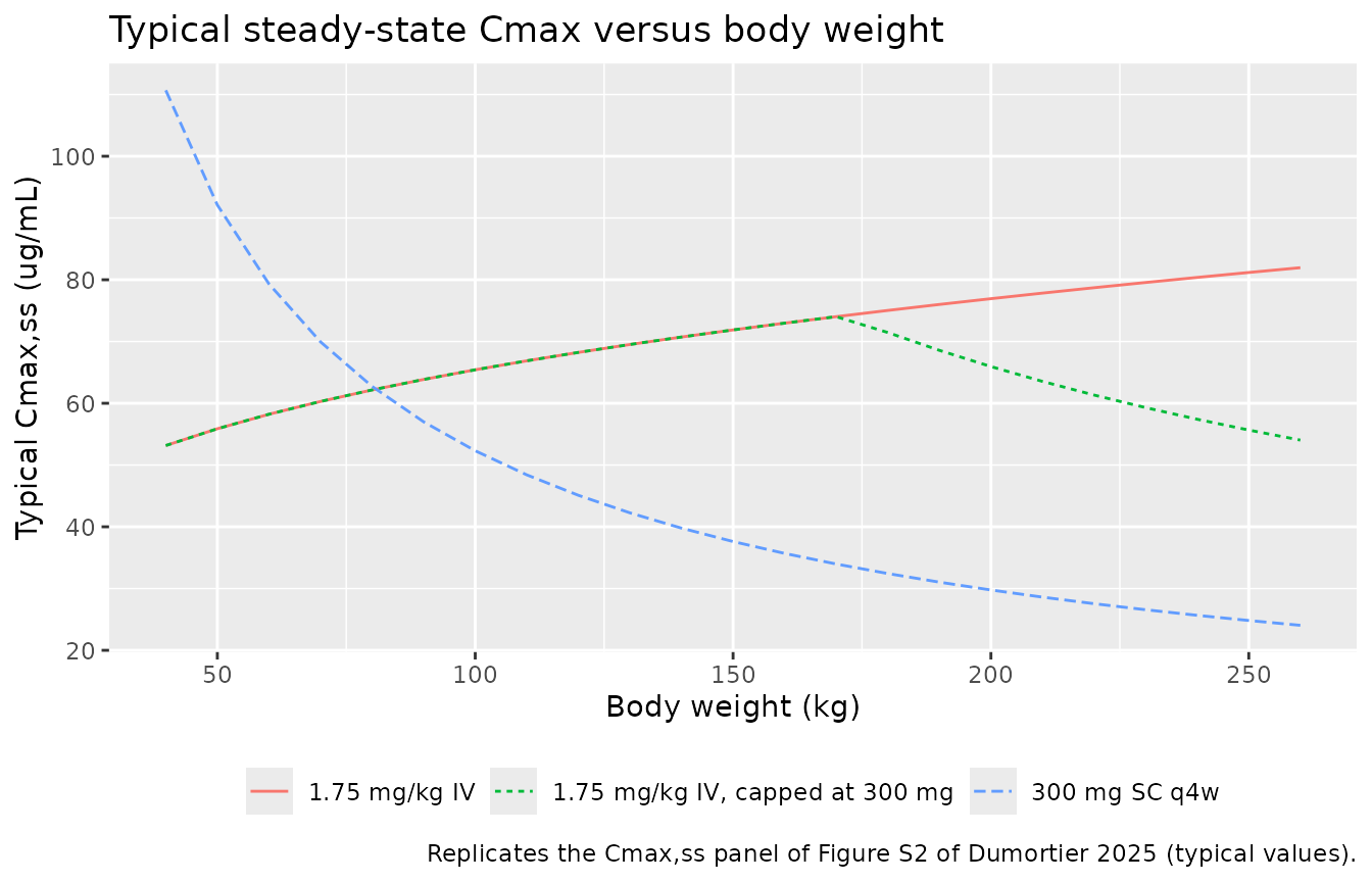
Figures S3, S4, S6 and S7 – exposure-response curves
conc_grid <- seq(0, 62, by = 0.5)
er_curve <- function(nm) {
  d <- data.frame(id = seq_along(conc_grid), time = 0, evid = 0, CTROUGH = conc_grid)
  s <- rxode2::rxSolve(er_ui[[nm]], d, returnType = "data.frame")
  tibble::tibble(model = nm, CTROUGH = conc_grid, p = s[[er_ui[[nm]]$predDf$var]])
}
curves <- dplyr::bind_rows(lapply(er_models$model, er_curve)) |>
  dplyr::left_join(er_models, by = "model")
#> Warning: multi-subject simulation without without 'omega'
#> Warning: multi-subject simulation without without 'omega'
#> Warning: multi-subject simulation without without 'omega'
#> Warning: multi-subject simulation without without 'omega'
#> Warning: multi-subject simulation without without 'omega'
#> Warning: multi-subject simulation without without 'omega'
#> Warning: multi-subject simulation without without 'omega'
#> Warning: multi-subject simulation without without 'omega'
#> Warning: multi-subject simulation without without 'omega'
#> Warning: multi-subject simulation without without 'omega'
#> Warning: multi-subject simulation without without 'omega'
#> Warning: multi-subject simulation without without 'omega'
#> Warning: multi-subject simulation without without 'omega'
#> Warning: multi-subject simulation without without 'omega'
#> Warning: multi-subject simulation without without 'omega'
#> Warning: multi-subject simulation without without 'omega'
#> Warning: multi-subject simulation without without 'omega'
#> Warning: multi-subject simulation without without 'omega'
#> Warning: multi-subject simulation without without 'omega'
#> Warning: multi-subject simulation without without 'omega'
#> Warning: multi-subject simulation without without 'omega'
#> Warning: multi-subject simulation without without 'omega'
#> Warning: multi-subject simulation without without 'omega'
#> Warning: multi-subject simulation without without 'omega'
#> Warning: multi-subject simulation without without 'omega'
#> Warning: multi-subject simulation without without 'omega'
#> Warning: multi-subject simulation without without 'omega'
#> Warning: multi-subject simulation without without 'omega'
#> Warning: multi-subject simulation without without 'omega'
#> Warning: multi-subject simulation without without 'omega'
#> Warning: multi-subject simulation without without 'omega'
#> Warning: multi-subject simulation without without 'omega'

ggplot(curves, aes(CTROUGH, p, colour = factor(week))) +
  geom_line() +
  facet_wrap(~ paste(disease, endpoint, sep = ": "), ncol = 4) +
  labs(
    x = "Pre-dose secukinumab concentration (ug/mL)", y = "Probability of response",
    colour = "Week",
    caption = "Replicates the fitted curves of Figures S3, S4 (Week 52) and S6, S7 (Week 16) of Dumortier 2025."
  ) +
  theme(strip.text = element_text(size = 7), legend.position = "bottom")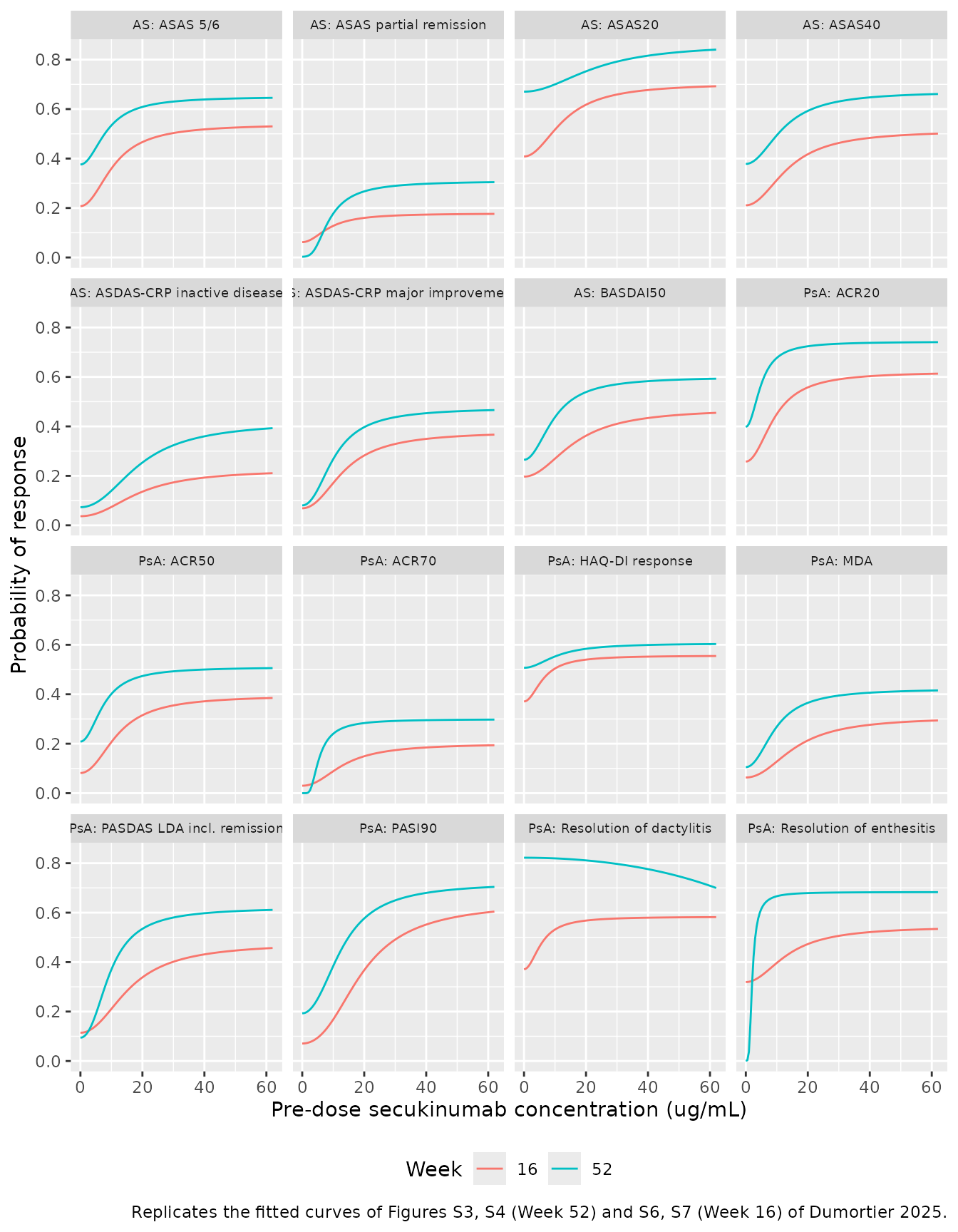
Predicted Week 52 efficacy of the IV and SC regimens
The Results section of Dumortier 2025 reports the mean predicted response probability at Week 52, averaged over the simulated Cmin,ss distribution of each regimen. The same calculation with the packaged PK and exposure-response models:
cmin_ss <- sim |>
  dplyr::filter(abs(time - (336 - 1e-3)) < 1e-6) |>
  dplyr::mutate(treatment = unname(ss_map[regimen])) |>
  dplyr::select(id, treatment, CTROUGH = Cc)

predict_mean <- function(nm) {
  d <- dplyr::mutate(cmin_ss, time = 0, evid = 0)
  s <- rxode2::rxSolve(er_ui[[nm]], d, keep = "treatment", returnType = "data.frame")
  s$p <- s[[er_ui[[nm]]$predDf$var]]
  dplyr::summarise(dplyr::group_by(s, treatment), simulated = 100 * mean(p), .groups = "drop") |>
    dplyr::mutate(model = nm)
}

published_w52 <- tibble::tribble(
  ~disease, ~token, ~`1.75 mg/kg IV q4w`, ~`150 mg SC q4w`, ~`300 mg SC q4w`,
  "PsA", "acr20", 72, 71, 74,
  "PsA", "acr50", 46, 45, 49,
  "PsA", "acr70", 27, 27, 29,
  "PsA", "haqdi", 58, 57, 59,
  "PsA", "dactylitis", 81, 81, 76,
  "PsA", "enthesitis", 67, 67, 68,
  "PsA", "pasi90", 54, 53, 65,
  "AS", "asas20", 74, 75, 80,
  "AS", "asas40", 57, 58, 64
) |>
  tidyr::pivot_longer(-c(disease, token), names_to = "treatment", values_to = "published") |>
  dplyr::mutate(model = sprintf("Dumortier_2025_secukinumab_%s_w52_%s", tolower(disease), token))

er_cmp <- dplyr::bind_rows(lapply(unique(published_w52$model), predict_mean)) |>
  dplyr::inner_join(published_w52, by = c("model", "treatment")) |>
  dplyr::left_join(dplyr::select(er_models, model, endpoint), by = "model") |>
  dplyr::mutate(diff = simulated - published)
#> Warning: multi-subject simulation without without 'omega'
#> Warning: multi-subject simulation without without 'omega'
#> Warning: multi-subject simulation without without 'omega'
#> Warning: multi-subject simulation without without 'omega'
#> Warning: multi-subject simulation without without 'omega'
#> Warning: multi-subject simulation without without 'omega'
#> Warning: multi-subject simulation without without 'omega'
#> Warning: multi-subject simulation without without 'omega'
#> Warning: multi-subject simulation without without 'omega'

er_cmp |>
  dplyr::select(disease, endpoint, treatment, published, simulated, diff) |>
  dplyr::rename("Disease" = disease, "Endpoint" = endpoint, "Regimen" = treatment,
                "Published (%)" = published, "Simulated (%)" = simulated,
                "Difference (points)" = diff) |>
knitr::kable(digits = 1, caption = "Mean predicted Week 52 response, simulated vs. Dumortier 2025 Results.")| Disease | Endpoint | Regimen | Published (%) | Simulated (%) | Difference (points) |
|---|---|---|---|---|---|
| PsA | ACR20 | 1.75 mg/kg IV q4w | 72 | 71.4 | -0.6 |
| PsA | ACR20 | 150 mg SC q4w | 71 | 71.4 | 0.4 |
| PsA | ACR20 | 300 mg SC q4w | 74 | 73.5 | -0.5 |
| PsA | ACR50 | 1.75 mg/kg IV q4w | 46 | 45.9 | -0.1 |
| PsA | ACR50 | 150 mg SC q4w | 45 | 46.0 | 1.0 |
| PsA | ACR50 | 300 mg SC q4w | 49 | 49.4 | 0.4 |
| PsA | ACR70 | 1.75 mg/kg IV q4w | 27 | 27.4 | 0.4 |
| PsA | ACR70 | 150 mg SC q4w | 27 | 27.5 | 0.5 |
| PsA | ACR70 | 300 mg SC q4w | 29 | 29.3 | 0.3 |
| PsA | HAQ-DI response | 1.75 mg/kg IV q4w | 58 | 57.8 | -0.2 |
| PsA | HAQ-DI response | 150 mg SC q4w | 57 | 57.8 | 0.8 |
| PsA | HAQ-DI response | 300 mg SC q4w | 59 | 59.6 | 0.6 |
| PsA | Resolution of dactylitis | 1.75 mg/kg IV q4w | 81 | 80.9 | -0.1 |
| PsA | Resolution of dactylitis | 150 mg SC q4w | 81 | 80.7 | -0.3 |
| PsA | Resolution of dactylitis | 300 mg SC q4w | 76 | 76.3 | 0.3 |
| PsA | Resolution of enthesitis | 1.75 mg/kg IV q4w | 67 | 67.6 | 0.6 |
| PsA | Resolution of enthesitis | 150 mg SC q4w | 67 | 67.6 | 0.6 |
| PsA | Resolution of enthesitis | 300 mg SC q4w | 68 | 68.2 | 0.2 |
| PsA | PASI90 | 1.75 mg/kg IV q4w | 54 | 54.3 | 0.3 |
| PsA | PASI90 | 150 mg SC q4w | 53 | 54.3 | 1.3 |
| PsA | PASI90 | 300 mg SC q4w | 65 | 65.9 | 0.9 |
| AS | ASAS20 | 1.75 mg/kg IV q4w | 74 | 74.8 | 0.8 |
| AS | ASAS20 | 150 mg SC q4w | 75 | 74.9 | -0.1 |
| AS | ASAS20 | 300 mg SC q4w | 80 | 80.5 | 0.5 |
| AS | ASAS40 | 1.75 mg/kg IV q4w | 57 | 57.6 | 0.6 |
| AS | ASAS40 | 150 mg SC q4w | 58 | 57.6 | -0.4 |
| AS | ASAS40 | 300 mg SC q4w | 64 | 63.6 | -0.4 |
Assumptions and deviations
-
Exposure-response parameters are figure-derived. No
E0, Emax or EC50 is printed anywhere in the paper or supplement. All 96
values were digitised by the maintainers from the fitted curves of
Figures S3, S4, S6 and S7 and refitted with the published equation (Hill
fixed at 2, as the paper states). The refit RMSE per panel is in each
model’s description. Three Week 52 PsA curves are only partly identified
by the plotted range:
- ACR70 and resolution of enthesitis: the curve is already near zero at the left edge of the plot, so E0 is only bounded from above; the least-squares optimum is reported.
-
Resolution of dactylitis: the curve decreases with exposure
and the plot shows only the start of the sigmoid, so EC50 and Emax are
not separately identifiable. EC50 was set to 400 ug/mL, on the ridge of
equally good fits (the limiting form over 0-62 ug/mL is
logit(p) = 1.529 - 1.785e-4 * Cmin^2). Do not extrapolate any of these three models beyond 0-62 ug/mL.
- Figure S3 HAQ-DI panel. Its y-axis labels read 0.0, 0.3, 0.4, 0.6 on equally spaced ticks; the “0.3” is a misprint for 0.2 (equal tick spacing of a linear axis) and the axis was calibrated as 0, 0.2, 0.4, 0.6.
- Endpoint definitions. Supplementary Table S2 lists “ASDAS-CRP major improvement” twice; the second row (“ASDAS-CRP score <= 1.3”) is ASDAS-CRP inactive disease, as the figure panels show. Table S2 defines PASDAS LDA as a score between 1.9 and 3.2, whereas the figure panels are titled “PASDAS LDA including remission”; the packaged output follows the figures.
-
CTROUGHinput. The exposure-response models take the pre-dose concentration at the assessment visit as a covariate. At Week 52 this is Cmin,ss; at Week 16 it is the Week 16 pre-dose concentration (0 for placebo patients). The models do not compute exposure themselves. - Placeholder residual. Each exposure-response model carries a fixed additive residual SD of 0.001 on the probability so nlmixr2 accepts the model; the source fits used a Bernoulli likelihood with no residual.
-
Fixed-to-zero random effects omitted. The control
stream declares
ETA(3)(Q),ETA(5)(KA) andETA(6)(logit F1) with variance0 FIX, and an additive residual0 FIX. They have no effect and are not carried. KA is fixed at 0.18/day as in the control stream and Table S3 (the Supplementary Methods text quotes 0.1801/day, the value estimated in psoriasis by Bruin 2017). - Weight effect on Q. The main text lists a weight effect on the intercompartmental flow, but neither the control stream nor Table S3 has one; Q is unscaled as in the control stream.
-
Final vs initial estimates. The
$THETA/$OMEGA/$SIGMAvalues in the supplementary control stream are initial estimates (e.g. CL 0.181); the packaged values are the final estimates of Table S3. - Simulation design. Infusion duration (30 minutes) and the body-weight distribution of the simulated INVIGORATE patients are not stated in the paper; a 30-minute infusion and a log-normal weight with mean 79 kg and SD 19 kg were used. Cohorts use 200 subjects per regimen instead of the paper’s 6000.
- Exposure-safety models not packaged. The Cox models with a penalised spline of the running-average concentration have a non-parametric baseline hazard and unreported spline coefficients.
- No erratum or correction notice was found for this article (Europe PMC, checked 2026-11-05).