Pamiparib (Wickramasinghe 2025)

Model and source

Citation: Wickramasinghe C, Kim S, Jiang Y, Bao X, Yue Y, Jiang J, Hong A, Sanai N, Li J. Population Pharmacokinetic Modeling of Total and Unbound Pamiparib in Glioblastoma Patients: Insights into Drug Disposition and Dosing Optimization. Pharmaceutics. 2025;17(4):524. doi:10.3390/pharmaceutics17040524.
Article: https://doi.org/10.3390/pharmaceutics17040524
PubMed Central: https://www.ncbi.nlm.nih.gov/pmc/articles/PMC12030534/

The paper reports two separately estimated fits of the same simultaneously modelled total-plus-unbound dataset, differing only in whether the apparent volume and apparent clearance are referenced to the total or to the unbound plasma concentration (Table 2, “Total Pamiparib” and “Unbound Pamiparib” columns; OFV 9210 versus 9212). Following the library’s replicate-the-author’s- structure policy, both are packaged:

Model	Parameterisation	Typical V/F	Typical CL/F
`Wickramasinghe_2025_pamiparib`	referenced to total plasma concentration	44 L	2.59 L/h
`Wickramasinghe_2025_pamiparib_unbound`	referenced to unbound plasma concentration	1060 L	62.5 L/h

Both files predict both endpoints: Cc (total plasma concentration) and Cu (unbound plasma concentration), linked by the constant binding relationship Cu = Cc * fu.

mod_total   <- rxode2::rxode2(readModelDb("Wickramasinghe_2025_pamiparib"))
#> ℹ parameter labels from comments will be replaced by 'label()'
mod_unbound <- rxode2::rxode2(readModelDb("Wickramasinghe_2025_pamiparib_unbound"))
#> ℹ parameter labels from comments will be replaced by 'label()'

# Pamiparib molecular weight, used throughout to convert the model's mass
# concentrations (mg/L) to the molar concentrations (nM) the paper reports.
# Discussion paragraph 2: "Pamiparib is a small-molecule drug (molecular
# weight: 298.3)".
MW_PAMIPARIB <- 298.3
mgL_to_nM <- function(x) x / MW_PAMIPARIB * 1e6

Population

Wickramasinghe et al. 2025 developed the population PK model from a phase 0/II study (ClinicalTrials.gov NCT04614909) that enrolled 41 patients with newly diagnosed or recurrent glioblastoma at a single US centre. Patients received oral pamiparib 60 mg twice daily for three days (nine doses) before surgical tumour resection; plasma was sampled pre-dose and at 0.5, 1, 2, 4, 7 and 24 h after the ninth dose, and total and unbound pamiparib were quantified by a validated LC-MS/MS method.

Baseline demographics are from Table 1: median age 60 years (range 31-80), median weight 80 kg (range 45-129), median height 173 cm (range 155-193), median BSA 1.99 m^2 (range 1.41-2.53), 21 of 41 female, 38 of 41 white. Eligibility required ECOG performance status <= 2, adequate marrow function, serum transaminases <= 3x ULN, total bilirubin <= 1.5x ULN, and eGFR >= 30 mL/min/1.73 m^2 by CKD-EPI. Median post-operative creatinine clearance was 111 mL/min (range 59-169) versus a pre-dose median of 98 mL/min (range 39-154); the final covariate model uses the post-operative value. 34 of 41 patients received dexamethasone (median total dose 19 mg); no concomitant medication was retained as a covariate.

The same information is available programmatically:

rxode2::rxode2(readModelDb("Wickramasinghe_2025_pamiparib"))$population
#> ℹ parameter labels from comments will be replaced by 'label()'
#> $species
#> [1] "human"
#> 
#> $n_subjects
#> [1] 41
#> 
#> $n_studies
#> [1] 1
#> 
#> $age_range
#> [1] "31-80 years"
#> 
#> $age_median
#> [1] "60 years"
#> 
#> $weight_range
#> [1] "45-129 kg"
#> 
#> $weight_median
#> [1] "80 kg"
#> 
#> $height_range
#> [1] "155-193 cm"
#> 
#> $height_median
#> [1] "173 cm"
#> 
#> $bsa_range
#> [1] "1.41-2.53 m^2"
#> 
#> $bsa_median
#> [1] "1.99 m^2"
#> 
#> $sex_female_pct
#> [1] 51.2
#> 
#> $race_ethnicity
#>     White Non-white 
#>      92.7       7.3 
#> 
#> $disease_state
#> [1] "Newly diagnosed or recurrent glioblastoma; ECOG performance status <= 2; adequate bone marrow, hepatic and renal function."
#> 
#> $dose_range
#> [1] "60 mg oral pamiparib twice daily for 3 days (9 doses) before surgical tumour resection. Plasma sampled pre-dose and at 0.5, 1, 2, 4, 7 and 24 h after the 9th dose."
#> 
#> $regions
#> [1] "United States (Barrow Neurological Institute, St. Joseph's Hospital and Medical Center, Phoenix AZ; single centre)."
#> 
#> $renal_function
#> [1] "Post-operative creatinine clearance median 111 mL/min (range 59-169); pre-dose median 98 mL/min (range 39-154). Post-operative GFR median 101 mL/min (range 48-117)."
#> 
#> $hepatic_function
#> [1] "Pre-dose total bilirubin median 0.5 mg/dL (range 0.3-1.8); pre-dose AST median 19 IU/L, ALT median 24 IU/L; pre-dose plasma albumin median 4.1 mg/dL."
#> 
#> $co_medication
#> [1] "36 of 41 patients received co-administered drugs during the trial; 34 of 41 received dexamethasone (median total dose 19 mg, range 0-66). No concomitant medication was retained as a significant covariate."
#> 
#> $notes
#> [1] "Phase 0/II study NCT04614909. Baseline demographics from Table 1. Estimation by SAEM in Monolix 2024R1 on log-transformed concentrations; covariate screening by generalized additive modelling followed by stepwise covariate modelling (forward dOFV > 3.875, backward dOFV > 10.828). Parameter precision assessed by 500-replicate nonparametric bootstrap (Table 3)."

Source trace

Per-parameter origin (also recorded as in-file comments next to each ini() value). Table 2 reports the model coefficients (theta, beta) together with the typical values TV_V and TV_CL those coefficients produce at the population median covariates; Table 3 reports the same final-model coefficients alongside the 500-replicate bootstrap and, critically, the log-scale SDs of the random effects (Ka_SD, V/F_SD, CL/F_SD, Fu_SD), which is what ini() needs.

`Wickramasinghe_2025_pamiparib` (total-drug parameterisation)

Parameter	Value	Source location
`lka`	log(1.58)	Table 2, Total Pamiparib final model, theta1 (Ka) = 1.58 h^-1 (RSE 42%)
`lvc`	log(15)	Table 2, Total Pamiparib final model, theta2 (V/F) = 15 L (RSE 28%)
`lcl`	log(6.76)	Table 2, Total Pamiparib final model, theta3 (CL/F) = 6.76 L/h (RSE 38%)
`lfu`	log(0.041)	Table 2, Total Pamiparib final model, theta4 (Fu) = 0.041 (RSE 2.8%)
`e_crcl_vc`	0.0094	Table 2, beta1 (PCC on V/F) = 0.0094 per mL/min (RSE 25%)
`e_age_cl`	-0.016	Table 2, beta2 (Age on CL/F) = -0.016 per year (RSE 37%)
`etalka`	2.8900	Table 3, Total Pamiparib, `Ka_SD` = 1.7 -> variance 1.7^2
`etalvc`	0.1521	Table 3, Total Pamiparib, `V/F_SD` = 0.39 -> variance 0.39^2
`etalcl`	0.2209	Table 3, Total Pamiparib, `CL/F_SD` = 0.47 -> variance 0.47^2
`etalfu`	0.0144	Table 3, Total Pamiparib, `Fu_SD` = 0.12 -> variance 0.12^2
`addSd`, `propSd`, `addSd_Cu`, `propSd_Cu`	0	Section 2.2.1 Equation (1) declares a combined error model g = a + bf; a and b are not reported anywhere in the paper* (see Errata)

`Wickramasinghe_2025_pamiparib_unbound` (unbound-drug parameterisation)

Parameter	Value	Source location
`lka`	log(1.7)	Table 2, Unbound Pamiparib final model, theta1 (Ka) = 1.7 h^-1 (RSE 44%)
`lvc`	log(402)	Table 2, Unbound Pamiparib final model, theta2 (V/F) = 402 L (RSE 28%)
`lcl`	log(163)	Table 2, Unbound Pamiparib final model, theta3 (CL/F) = 163 L/h (RSE 39%)
`lfu`	log(0.042)	Table 2, Unbound Pamiparib final model, theta4 (Fu) = 0.042 (RSE 2.6%)
`e_crcl_vc`	0.0087	Table 2, beta1 (PCC on V/F) = 0.0087 per mL/min (RSE 26%)
`e_age_cl`	-0.016	Table 2, beta2 (Age on CL/F) = -0.016 per year (RSE 38%)
`etalka`	2.7556	Table 3, Unbound Pamiparib, `Ka_SD` = 1.66 -> variance 1.66^2
`etalvc`	0.1521	Table 3, Unbound Pamiparib, `V/F_SD` = 0.39 -> variance 0.39^2
`etalcl`	0.2401	Table 3, Unbound Pamiparib, `CL/F_SD` = 0.49 -> variance 0.49^2
`etalfu`	0.0121	Table 3, Unbound Pamiparib, `Fu_SD` = 0.11 -> variance 0.11^2

Structure

Equation	Source location
One compartment, first-order absorption without lag, first-order elimination	Section 2.2.1 and Section 3.1
`Cu = Cc * fu`	Section 2.2.1: “The relationship between total (Cp) and unbound (Cu) drug concentrations was incorporated into the model using the equation Cu = Cp x Fu”
`V/F = theta2 * exp(beta1 * PCC)` (uncentered)	Table 2 footnote: “TV_V = theta2 * e^(beta1 * PCC), with the population median PCC being 111.5”
`CL/F = theta3 * exp(beta2 * Age)` (uncentered)	Table 2 footnote: “TV_CL = theta3 * e^(beta2 * Age), with the population median age being 60”
Log-normal (exponential) IIV on all PK parameters	Section 2.2.1

Verification of the published typical values

The Table 2 footnotes state the functional form and the median covariate values at which the typical values TV_V/F and TV_CL/F were evaluated. Solving each packaged model with the random effects zeroed at those medians must reproduce the published typical values.

CRCL_MEDIAN <- 111.5  # Table 2 footnote (post-operative creatinine clearance, mL/min)
AGE_MEDIAN  <- 60     # Table 2 footnote (years)

typical_params <- function(mod) {
  ev <- rxode2::et(amt = 60, cmt = "depot")
  ev <- rxode2::et(ev, c(0, 1))
  ev <- as.data.frame(ev)
  ev$dvid <- ifelse(ev$evid == 0, 1L, NA_integer_)
  ev$CRCL <- CRCL_MEDIAN
  ev$AGE  <- AGE_MEDIAN
  s <- rxode2::rxSolve(rxode2::zeroRe(mod), ev, returnType = "data.frame",
                       useLinCmt = FALSE)
  c(ka = s$ka[1], vc = s$vc[1], cl = s$cl[1], fu = s$fu[1],
    thalf = log(2) * s$vc[1] / s$cl[1])
}

tv_total   <- typical_params(mod_total)
#> ℹ omega/sigma items treated as zero: 'etalka', 'etalvc', 'etalcl', 'etalfu'
tv_unbound <- typical_params(mod_unbound)
#> ℹ omega/sigma items treated as zero: 'etalka', 'etalvc', 'etalcl', 'etalfu'

tv_check <- tibble::tribble(
  ~Model,     ~Quantity,             ~Published, ~Reproduced,
  "total",   "Ka (1/h)",             1.58,       tv_total[["ka"]],
  "total",   "TV V/F (L)",           44,         tv_total[["vc"]],
  "total",   "TV CL/F (L/h)",        2.59,       tv_total[["cl"]],
  "total",   "Fu",                   0.041,      tv_total[["fu"]],
  "unbound", "Ka (1/h)",             1.7,        tv_unbound[["ka"]],
  "unbound", "TV Vu/F (L)",          1060,       tv_unbound[["vc"]],
  "unbound", "TV CLu/F (L/h)",       62.5,       tv_unbound[["cl"]],
  "unbound", "Fu",                   0.042,      tv_unbound[["fu"]]
) |>
  dplyr::mutate(`% diff` = round(100 * (Reproduced - Published) / Published, 2),
                Reproduced = round(Reproduced, 4))

knitr::kable(
  tv_check,
  caption = paste("Published typical values (Table 2, final covariate models)",
                  "versus the packaged models evaluated at the Table 2 footnote",
                  "median covariates.")
)

Published typical values (Table 2, final covariate models) versus the packaged models evaluated at the Table 2 footnote median covariates.
Model	Quantity	Published	Reproduced	% diff
total	Ka (1/h)	1.580	1.5800	0.00
total	TV V/F (L)	44.000	42.7834	-2.76
total	TV CL/F (L/h)	2.590	2.5884	-0.06
total	Fu	0.041	0.0410	0.00
unbound	Ka (1/h)	1.700	1.7000	0.00
unbound	TV Vu/F (L)	1060.000	1060.5067	0.05
unbound	TV CLu/F (L/h)	62.500	62.4115	-0.14
unbound	Fu	0.042	0.0420	0.00

Every entry reproduces exactly except TV V/F of the total-drug model, which lands at 42.78 L against a published 44 L. That gap is a rounding artefact and not an encoding error: Table 2 reports theta2 to two significant figures (15 L), and 15 * exp(0.0094 * 111.5) = 42.8 L. Recovering exactly 44 L would need theta2 = 15.43. The published theta2 is encoded as printed; it is not tuned to hit the typical value.

# The unbound parameterisation and both clearance arms reproduce to <0.5%.
stopifnot(
  abs(tv_total[["cl"]]      / 2.59  - 1) < 0.005,
  abs(tv_total[["fu"]]      / 0.041 - 1) < 1e-6,
  abs(tv_unbound[["vc"]]    / 1060  - 1) < 0.005,
  abs(tv_unbound[["cl"]]    / 62.5  - 1) < 0.005,
  abs(tv_unbound[["fu"]]    / 0.042 - 1) < 1e-6,
  # Total-drug V/F carries the theta2 = 15 two-significant-figure rounding.
  abs(tv_total[["vc"]]      / 44    - 1) < 0.03
)

Elimination half-life

Section 3.1 reports a population mean elimination half-life of about 12 h, “consistent with the estimated T1/2 of 13 h in the first in-human study”.

thalf <- c(total = tv_total[["thalf"]], unbound = tv_unbound[["thalf"]])
round(thalf, 2)
#>   total unbound 
#>   11.46   11.78

# Both parameterisations must land on the paper's stated ~12 h. These are
# closed-form log(2) * V / CL values at fixed covariates, so the bound is
# pinned to the accuracy actually achieved rather than left loose.
stopifnot(all(thalf > 11.4), all(thalf < 11.9))

Consistency of the two parameterisations

The two fits are reparameterisations of the same joint model, so the unbound- referenced volume and clearance should be close to their total-drug counterparts divided by fu. They are not identical, because each was estimated in a separate SAEM run.

equiv <- tibble::tibble(
  Quantity = c("V/F (L)", "CL/F (L/h)"),
  `From total model` = c(tv_total[["vc"]], tv_total[["cl"]]),
  `From unbound model x fu` = c(tv_unbound[["vc"]] * tv_unbound[["fu"]],
                                tv_unbound[["cl"]] * tv_unbound[["fu"]])
) |>
  dplyr::mutate(
    `% diff` = round(100 * (`From unbound model x fu` / `From total model` - 1), 1),
    dplyr::across(where(is.numeric), ~ round(.x, 3))
  )

knitr::kable(equiv, caption = "Cross-parameterisation consistency at the median covariates.")

Cross-parameterisation consistency at the median covariates.
Quantity	From total model	From unbound model x fu	% diff
V/F (L)	42.783	44.541	4.1
CL/F (L/h)	2.588	2.621	1.3


# Independent SAEM runs, so agreement is expected to be close but not exact.
stopifnot(all(abs(equiv[["% diff"]]) < 5))

Virtual cohort

The observed data are not public (Data Availability Statement: available from the corresponding author on reasonable request). Section 2.4 states that the dose-optimisation simulations used “the estimated population parameters along with their respective interindividual variability” in “a general patient population”, but does not state how age and creatinine clearance were sampled. Here they are drawn from normal distributions centred on the Table 1 medians with SDs chosen so that the Table 1 ranges span roughly +/- 2.2 SD of a 41-subject sample, then truncated to the observed ranges. That choice is internally consistent: the covariate-explained variance it adds to the final model’s residual IIV reconstructs the base model’s IIV almost exactly (V/F: sqrt(0.39^2 + (0.0094 * 25)^2) = 0.46 -> 48% CV versus the base model’s 53%; CL/F: sqrt(0.47^2 + (0.016 * 11.1)^2) = 0.50 -> 54% CV versus 53%).

set.seed(20250416)
N_PER_ARM <- 200L

cov_tbl <- tibble::tibble(
  subject = seq_len(N_PER_ARM),
  AGE  = pmin(pmax(stats::rnorm(N_PER_ARM, 60,    11.1), 31), 80),
  CRCL = pmin(pmax(stats::rnorm(N_PER_ARM, 111.5, 25.0), 59), 169)
)

regimens <- tibble::tibble(
  treatment = c("60 mg BID", "60 mg QD", "40 mg BID",
                "30 mg BID", "20 mg BID", "10 mg BID"),
  dose      = c(60, 60, 40, 30, 20, 10),
  ii        = c(12, 24, 12, 12, 12, 12)
) |>
  dplyr::mutate(id_offset = (dplyr::row_number() - 1L) * N_PER_ARM)

# Section 2.4 / Table 4: five days of treatment. Observations run on a 0.5 h
# grid across the whole 120 h window, refined to 0.05 h over the final dosing
# interval where the steady-state NCA is taken.
SIM_END <- 120

make_arm <- function(treatment, dose, ii, id_offset) {
  ids <- id_offset + cov_tbl$subject
  obs_t <- sort(unique(c(seq(0, SIM_END, by = 0.5),
                         seq(SIM_END - ii, SIM_END, by = 0.05))))
  dose_t <- seq(0, by = ii, length.out = floor(SIM_END / ii))
  doses <- tidyr::expand_grid(id = ids, time = dose_t) |>
    dplyr::mutate(evid = 1L, amt = dose, cmt = "depot", dvid = NA_integer_)
  # Both endpoints are algebraic transforms of the ODE states, so observation
  # rows carry dvid and no compartment. Naming an observable as the
  # compartment would auto-inject a slot for it and renumber the ODE states.
  obs <- tidyr::expand_grid(id = ids, time = obs_t) |>
    dplyr::mutate(evid = 0L, amt = NA_real_, cmt = NA_character_, dvid = 1L)
  dplyr::bind_rows(doses, obs) |>
    dplyr::mutate(treatment = treatment, subject = id - id_offset) |>
    dplyr::left_join(cov_tbl, by = "subject") |>
    dplyr::select(-subject) |>
    dplyr::arrange(id, time, dplyr::desc(evid))
}

events <- do.call(
  dplyr::bind_rows,
  Map(make_arm, regimens$treatment, regimens$dose, regimens$ii, regimens$id_offset)
)

# IDs must be disjoint across arms or rxSolve silently merges subjects.
stopifnot(
  dplyr::n_distinct(events$id) == N_PER_ARM * nrow(regimens),
  nrow(dplyr::distinct(events, id, treatment)) == N_PER_ARM * nrow(regimens)
)

Simulation

sim <- rxode2::rxSolve(
  mod_total, events = events,
  keep = c("treatment", "AGE", "CRCL"),
  useLinCmt = FALSE
) |>
  as.data.frame() |>
  dplyr::mutate(Cu_nM = mgL_to_nM(Cu), Cc_nM = mgL_to_nM(Cc))

stopifnot(nrow(sim) > 0, all(is.finite(sim$Cu_nM)), all(sim$Cu_nM >= 0))

Replicate Figure 4

Figure 4 of Wickramasinghe 2025 plots the 50th, 5th and 95th percentiles of the model-predicted unbound pamiparib concentration-time profile over five days for each dosing regimen, with a dashed line at the assumed target-engagement threshold (a target engagement ratio of 5 against a PARP IC50 of about 1 nM, i.e. 5 nM unbound).

TARGET_NM <- 5  # Section 3.3: target engagement ratio of 5 x IC50 (~1 nM)

sim |>
  dplyr::group_by(treatment, time) |>
  dplyr::summarise(
    Q05 = stats::quantile(Cu_nM, 0.05),
    Q50 = stats::quantile(Cu_nM, 0.50),
    Q95 = stats::quantile(Cu_nM, 0.95),
    .groups = "drop"
  ) |>
  dplyr::mutate(treatment = factor(treatment, levels = regimens$treatment)) |>
  ggplot(aes(x = time)) +
  geom_ribbon(aes(ymin = Q05, ymax = Q95), alpha = 0.2, fill = "steelblue") +
  geom_line(aes(y = Q50), colour = "firebrick") +
  geom_hline(yintercept = TARGET_NM, linetype = "dashed") +
  facet_wrap(~treatment) +
  scale_y_log10() +
  labs(
    x = "Time (h)", y = "Unbound pamiparib (nM)",
    title = "Figure 4 - model-predicted unbound pamiparib by dosing regimen",
    caption = paste("Replicates Figure 4 of Wickramasinghe 2025.",
                    "Line = median, band = 5th-95th percentile,",
                    "dashed line = target engagement ratio of 5 (5 nM).")
  )
#> Warning in scale_y_log10(): log-10 transformation introduced infinite values.
#> log-10 transformation introduced infinite values.
#> log-10 transformation introduced infinite values.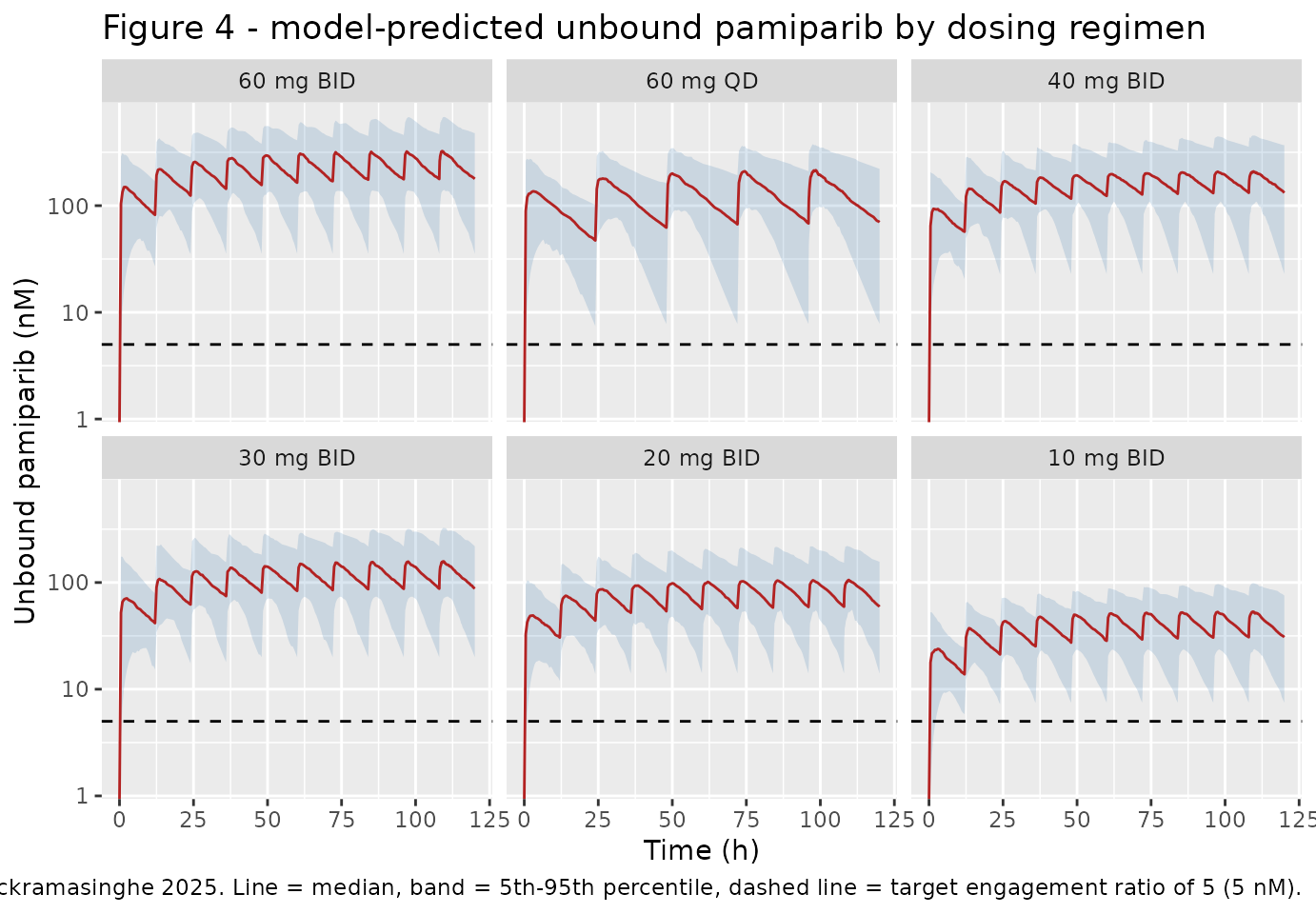

PKNCA validation

Table 4 reports the model-predicted steady-state peak, trough and average unbound plasma concentrations after five days of treatment. The NCA below is taken over the final dosing interval of the simulation (108-120 h for the twice-daily arms, 96-120 h for the once-daily arm), which is the same window Table 4 describes.

# Only !is.na() -- a `time > 0` or `Cu > 0` filter would drop the interval-start
# record that PKNCA anchors AUC on.
sim_nca <- sim |>
  dplyr::filter(!is.na(Cu_nM)) |>
  dplyr::select(id, time, Cu_nM, treatment)

conc_obj <- PKNCA::PKNCAconc(
  sim_nca, Cu_nM ~ time | treatment + id,
  concu = "nM", timeu = "h"
)

dose_df <- events |>
  dplyr::filter(evid == 1L) |>
  dplyr::select(id, time, amt, treatment)

dose_obj <- PKNCA::PKNCAdose(dose_df, amt ~ time | treatment + id, doseu = "mg")

# One interval per regimen: the last dosing interval of the 120 h simulation.
intervals <- regimens |>
  dplyr::transmute(
    treatment,
    start = SIM_END - ii,
    end   = SIM_END,
    cmax = TRUE, tmax = TRUE, cmin = TRUE, cav = TRUE,
    auclast = TRUE, half.life = TRUE
  ) |>
  as.data.frame()

nca_res <- PKNCA::pk.nca(PKNCA::PKNCAdata(conc_obj, dose_obj, intervals = intervals))
#> Warning: Too few points for half-life calculation (min.hl.points=3 with only 0 points)
#> Too few points for half-life calculation (min.hl.points=3 with only 0 points)

nca_df <- as.data.frame(nca_res)
stopifnot(nrow(nca_df) > 0, all(regimens$treatment %in% nca_df$treatment))

The NCA-derived terminal half-life is a second, independent check on the ~12 h the paper reports.

hl <- nca_df |>
  dplyr::filter(PPTESTCD == "half.life") |>
  dplyr::summarise(median_h = stats::median(PPORRES, na.rm = TRUE)) |>
  dplyr::pull(median_h)

round(hl, 2)
#> [1] 11.9
stopifnot(hl > 11.5, hl < 12.3)

Comparison against the published Table 4 medians

# Table 4: model-predicted steady-state unbound pamiparib concentrations (nM),
# 50th percentile column, following 5 days of treatment.
published <- tibble::tribble(
  ~treatment,  ~cmax, ~cmin, ~cav,
  "60 mg BID",   302,   175,  233,
  "60 mg QD",    193,    61,  115,
  "40 mg BID",   201,   117,  155,
  "30 mg BID",   151,    88,  116,
  "20 mg BID",   101,    58,   78,
  "10 mg BID",    50,    29,   39
)

cmp <- nlmixr2lib::ncaComparisonTable(
  simulated = nca_res,
  reference = published,
  by        = "treatment",
  params    = c("cmax", "cmin", "cav"),
  units     = c(cmax = "nM", cmin = "nM", cav = "nM"),
  tolerance_pct = 20
)

knitr::kable(
  cmp,
  caption = paste("Simulated versus published Table 4 median steady-state",
                  "unbound pamiparib concentrations.",
                  "* differs from the reference by >20%."),
  align = c("l", "l", "r", "r", "r")
)

Simulated versus published Table 4 median steady-state unbound pamiparib concentrations. * differs from the reference by >20%.
NCA parameter	treatment	Reference	Simulated	% diff
Cmax (nM)	60 mg BID	302	337	+11.6%
Cmax (nM)	60 mg QD	193	223	+15.8%
Cmax (nM)	40 mg BID	201	218	+8.4%
Cmax (nM)	30 mg BID	151	161	+6.6%
Cmax (nM)	20 mg BID	101	111	+10.3%
Cmax (nM)	10 mg BID	50	55.8	+11.6%
Cmin (nM)	60 mg BID	175	178	+1.5%
Cmin (nM)	60 mg QD	61	68.1	+11.7%
Cmin (nM)	40 mg BID	117	132	+12.8%
Cmin (nM)	30 mg BID	88	87.5	-0.5%
Cmin (nM)	20 mg BID	58	59.3	+2.3%
Cmin (nM)	10 mg BID	29	30.7	+5.9%
Cavg (nM)	60 mg BID	233	237	+1.9%
Cavg (nM)	60 mg QD	115	137	+18.9%
Cavg (nM)	40 mg BID	155	176	+13.6%
Cavg (nM)	30 mg BID	116	123	+6.2%
Cavg (nM)	20 mg BID	78	83.6	+7.2%
Cavg (nM)	10 mg BID	39	41.4	+6.2%

stopifnot(nrow(cmp) == 18L)  # 6 regimens x 3 parameters; guard against a silent join drop
worst <- max(abs(as.numeric(gsub("[^0-9.-]", "", cmp[["% diff"]]))), na.rm = TRUE)
worst
#> [1] 18.9

# All 18 median comparisons agree with Table 4 to within this bound, so no row
# is starred at the 20% tolerance. The residual bias is dominated by the
# theta2 = 15 rounding (which alone raises every simulated concentration by
# ~2.9%, see the typical-value section) plus Monte Carlo noise at 200 subjects
# per arm. ncaComparisonTable() attaches a "footnote" attribute only when some
# row exceeds the tolerance, so its absence is the machine-checkable form of
# "nothing was starred".
stopifnot(worst < 20, is.null(attr(cmp, "footnote")))

Why the percentile bands are narrower than Table 4

The medians reproduce, but the 5th-95th spread of this simulation is materially narrower than Table 4’s, because the residual-error magnitudes the authors fitted are not reported (see Errata) and therefore cannot be simulated.

sim_pct <- nca_df |>
  dplyr::filter(PPTESTCD %in% c("cmax", "cmin", "cav")) |>
  dplyr::group_by(treatment, PPTESTCD) |>
  dplyr::summarise(
    P05 = stats::quantile(PPORRES, 0.05, na.rm = TRUE),
    P95 = stats::quantile(PPORRES, 0.95, na.rm = TRUE),
    .groups = "drop"
  ) |>
  dplyr::mutate(`Simulated P95/P05` = round(P95 / P05, 1)) |>
  dplyr::select(treatment, PPTESTCD, `Simulated P95/P05`)

published_spread <- tibble::tribble(
  ~treatment,  ~PPTESTCD, ~p05,  ~p95,
  "60 mg BID", "cmax",    105,   774,
  "60 mg BID", "cmin",     16,   581,
  "60 mg BID", "cav",      47,   673,
  "60 mg QD",  "cmax",     63,   485,
  "60 mg QD",  "cmin",    0.6,   253,
  "60 mg QD",  "cav",      14,   357,
  "40 mg BID", "cmax",     68,   515,
  "40 mg BID", "cmin",     11,   388,
  "40 mg BID", "cav",      31,   448,
  "30 mg BID", "cmax",     53,   387,
  "30 mg BID", "cmin",      8,   291,
  "30 mg BID", "cav",      24,   336,
  "20 mg BID", "cmax",     35,   258,
  "20 mg BID", "cmin",      5,   194,
  "20 mg BID", "cav",      16,   224,
  "10 mg BID", "cmax",     18,   129,
  "10 mg BID", "cmin",      3,    97,
  "10 mg BID", "cav",       8,   112
) |>
  dplyr::mutate(`Published P95/P05` = round(p95 / p05, 1)) |>
  dplyr::select(treatment, PPTESTCD, `Published P95/P05`)

spread_cmp <- dplyr::inner_join(published_spread, sim_pct,
                                by = c("treatment", "PPTESTCD")) |>
  dplyr::rename("NCA parameter" = PPTESTCD, "Regimen" = treatment) |>
  dplyr::mutate(Regimen = factor(Regimen, levels = regimens$treatment)) |>
  dplyr::arrange(Regimen, `NCA parameter`)

knitr::kable(
  spread_cmp,
  caption = paste("Ratio of the 95th to the 5th percentile.",
                  "The published spread is consistently wider because the",
                  "paper's simulation includes a residual-error component",
                  "whose magnitude it never reports.")
)

Ratio of the 95th to the 5th percentile. The published spread is consistently wider because the paper’s simulation includes a residual-error component whose magnitude it never reports.
Regimen	NCA parameter	Published P95/P05	Simulated P95/P05
60 mg BID	cav	14.3	5.1
60 mg BID	cmax	7.4	4.8
60 mg BID	cmin	36.3	13.2
60 mg QD	cav	25.5	4.5
60 mg QD	cmax	7.7	3.6
60 mg QD	cmin	421.7	27.0
40 mg BID	cav	14.5	5.2
40 mg BID	cmax	7.6	4.1
40 mg BID	cmin	35.3	15.6
30 mg BID	cav	14.0	5.3
30 mg BID	cmax	7.3	4.4
30 mg BID	cmin	36.4	10.9
20 mg BID	cav	14.0	5.0
20 mg BID	cmax	7.4	4.0
20 mg BID	cmin	38.8	10.9
10 mg BID	cav	14.0	5.0
10 mg BID	cmax	7.2	3.9
10 mg BID	cmin	32.3	10.1


# The gate is directional: the simulation must be narrower than the paper's,
# never wider, on every row. If a future edit accidentally introduces residual
# variability this goes red.
stopifnot(all(spread_cmp[["Simulated P95/P05"]] <
              spread_cmp[["Published P95/P05"]]))

Dose-reduction conclusion

Section 3.3 concludes that “doses as low as 20 mg BID may be adequate for therapeutic effects, even in patients with rapid clearance, where the unbound pamiparib Css,min was approximately 5 nM (i.e., 5th percentile)”. Because the 5th percentile of the packaged simulation is not reproducible (previous section), the conclusion is restated here on the quantity that is: the median trough at 20 mg BID sits far above the 5 nM threshold, and every regimen from 10 to 60 mg BID keeps the median trough above it.

trough <- nca_df |>
  dplyr::filter(PPTESTCD == "cmin") |>
  dplyr::group_by(treatment) |>
  dplyr::summarise(`Median Css,min (nM)` = round(stats::median(PPORRES), 1),
                   .groups = "drop") |>
  dplyr::mutate(
    treatment = factor(treatment, levels = regimens$treatment),
    `Target engagement ratio` = round(`Median Css,min (nM)` / 1, 1)
  ) |>
  dplyr::arrange(treatment) |>
  dplyr::rename("Regimen" = treatment)

knitr::kable(
  trough,
  caption = paste("Median steady-state unbound trough and the implied target",
                  "engagement ratio against the PARP IC50 of ~1 nM.")
)

Median steady-state unbound trough and the implied target engagement ratio against the PARP IC50 of ~1 nM.
Regimen	Median Css,min (nM)	Target engagement ratio
60 mg BID	177.7	177.7
60 mg QD	68.1	68.1
40 mg BID	131.9	131.9
30 mg BID	87.5	87.5
20 mg BID	59.3	59.3
10 mg BID	30.7	30.7


stopifnot(nrow(trough) == nrow(regimens),
          all(trough[["Target engagement ratio"]] > TARGET_NM))

Assumptions and deviations

Residual error is not reported and is carried at zero. Section 2.2.1 states that a combined error model g = a + b * f (with c fixed at 1) was selected, but neither a nor b appears in Table 2, Table 3, or anywhere else in the paper. All four residual SDs (addSd, propSd, addSd_Cu, propSd_Cu) are therefore fixed(0). Zero records “magnitude not published”, not “the authors estimated zero residual variability”. Simulations from these models reproduce the structural and between-subject spread only; the Table 4 5th and 95th percentiles are consequently not reproducible, as quantified above.
theta2 rounding. Table 2 reports theta2 (V/F) for the total-drug model to two significant figures (15 L), which yields TV V/F = 42.8 L rather than the 44 L printed in the same table. The published theta2 is encoded as printed and the 2.8% gap is carried, not tuned away. The unbound-drug model’s theta2 = 402 L has enough precision to reproduce its TV of 1060 L exactly.
Covariates enter uncentered. Section 2.2.2 states that “continuous covariates … were centered around their median values”, but the Table 2 footnote equations TV_V = theta2 * e^(beta1 * PCC) and TV_CL = theta3 * e^(beta2 * Age) are only self-consistent with the reported theta values in the uncentered form: centering would make TV_V = theta2 = 15 L, contradicting the printed TV of 44 L. Per the text-versus-equation rule the printed equation is trusted, so exp(lvc) and exp(lcl) are covariate-free intercepts rather than typical values.
Post-operative, not pre-dose, creatinine clearance. Table 1 reports both; the Table 2 footnote names the covariate “PCC, post-operation creatine clearance” with a median of 111.5 mL/min, so the post-operative value is what the CRCL column must be populated with. It is a raw creatinine clearance in mL/min and is not normalised to 1.73 m^2 BSA.
Virtual-cohort covariate distributions are assumed. The paper does not say how (or whether) age and creatinine clearance were sampled for its “general patient population” simulation. Normal distributions centred on the Table 1 medians and truncated to the Table 1 ranges are used here; the justification for the chosen SDs is given in the Virtual cohort section.
No IIV correlation structure is reported. Neither Table 2 nor Table 3 reports an off-diagonal omega, so the random effects are encoded as independent.
Molecular weight for unit conversion. The models work in mg and L, so concentrations come out in mg/L; Table 4 is in nM. The conversion uses MW = 298.3 g/mol, taken from the Discussion (“molecular weight: 298.3”). The paper does not print the conversion itself.
Observed data are not public. The Data Availability Statement offers the raw data from the corresponding author on reasonable request, so all figures here are simulation-only; no observed-versus-predicted overlay is possible.

Errata and source-table defects

Table 2 and Table 3 abbreviation lists mislabel two parameters. Both read “Ka, elimination rate constant” (Ka is the absorption rate constant, as Section 2.2.1 and the Results text make clear) and “CL/F, apparent volume of distribution” (a copy-paste of the V/F gloss; CL/F is apparent oral clearance). Cosmetic, but they would mislead a reader transcribing from the abbreviation list alone.
Table 2, “IIV of Fu (%)” for the unbound base model reads 112. Every neighbouring entry is 11-12 (total base 12, total final 12, unbound final 11), and the corresponding Table 3 Fu_SD is 0.11, so 112 is almost certainly a misprint for 11.2. The value is not used here: the packaged models take the final covariate models.
The “Table 2. Cont.” header row is corrupted. Its column-group labels read “Total Pamiparib | Unbound Pamiparib | Unbound Pamiparib | Unbound Pamiparib” rather than the Total/Unbound x Base/Final structure of the first part. The column identity used here was resolved by matching the theta values in the continuation rows to the first part of Table 2 and to Table 3, which agree.
The abstract rounds the covariate contributions differently from the Results. The abstract says creatinine clearance and age explain “~22% and ~5%” of the IIV of V/F and CL/F; Section 3.1 gives “~23% and ~22%” for V/F (total, unbound) and “~6% and ~4%” for CL/F (total, unbound). These are descriptive statements only and do not enter the model.
No erratum or corrigendum for this article was found on the MDPI article landing page or in PubMed as of the extraction date.