Darunavir external validation (Stillemans 2021b)
Source:vignettes/articles/Stillemans_2021b_darunavir.Rmd
Stillemans_2021b_darunavir.RmdModel and source
- Citation: Stillemans G, Belkhir L, Vandercam B, Vincent A, Haufroid V, Elens L. Optimal sampling strategies for darunavir and external validation of the underlying population pharmacokinetic model. Eur J Clin Pharmacol. 2021;77(4):607-616. doi:10.1007/s00228-020-03036-2. PMCID: PMC7935830.
- Description: One-compartment population pharmacokinetic model with first-order absorption and elimination for oral ritonavir- or cobicistat-boosted darunavir in adults with HIV-1 infection, re-estimated on the merged learning and external-validation datasets (Stillemans 2021, Eur J Clin Pharmacol). Reduced covariate model without alpha-1 acid glycoprotein: apparent clearance is lower in women and in CYP3A5 nonexpressers (3/3); apparent volume is higher in SLCO3A1 rs8027174 G>T carriers.
- Article: https://doi.org/10.1007/s00228-020-03036-2 (open access, PMC7935830)
- Electronic supplementary material: Supplementary Material 1 of the article (full versus reduced model on the learning set, with RSE and shrinkage).
- Underlying model: Stillemans 2021, Clin Pharmacokinet 60:177-189 (https://doi.org/10.1007/s40262-020-00920-z), whose ESM Online Resource 2 gives the covariate equation forms.
This paper externally validates the authors’ earlier population PK model of boosted darunavir and then uses it to derive optimal sampling strategies. The validation cohort had no alpha-1 acid glycoprotein (AAG) measurements, so the authors removed AAG from the model and validated this reduced model instead. After validation they merged the learning and validation data and re-estimated the reduced model. That re-estimate (Table 2, “Merged set”) is the model packaged here. The learning-set estimates of the same reduced model (Table 2, “Learning set”) are compared with it below.
The structure is a one-compartment model with first-order absorption and first-order elimination. Apparent clearance (CL/F) is lower in women (exponential effect) and in CYP3A5 nonexpressers (*3/*3; categorical). Apparent volume (V/F) is larger in SLCO3A1 rs8027174 G>T carriers (categorical).
Population
The learning set is the companion study: 127 adults with HIV-1 and 405 darunavir concentrations. Most were cobicistat-boosted (85.8%) and took 800 mg once daily (91.3%). Twelve patients contributed 6-hour rich profiles. The validation set held 164 adults, all ritonavir-boosted, sampled once per dosing interval at random post-intake times between November 2012 and April 2016. That gave 180 samples, one of them excluded for an unknown post-intake time. The validation patients took 800 mg once daily (67.1%) or 600 mg twice daily (29.3%). They were younger than the learning set (median 48 vs 55 years) and sampled later after the dose (median 14.8 vs 6.3 h). Sex, race and genotype frequencies did not differ significantly (Table 1). Fifty-one patients were in both studies, and the merged fit treated their two studies as separate occasions.
str(rxode2::rxode(readModelDb("Stillemans_2021b_darunavir"))$population)
#> ℹ parameter labels from comments will be replaced by 'label()'
#> List of 13
#>  $ species       : chr "human"
#>  $ n_subjects    : num 291
#>  $ n_studies     : num 2
#>  $ n_observations: num 584
#>  $ age_median    : chr "55 years (IQR 13) learning set; 48 years (IQR 14) validation set (Table 1)"
#>  $ sex_female_pct: num 34.7
#>  $ race_ethnicity: chr "Learning set Caucasian 52.8%, African 43.3%; validation set Caucasian 61.6%, African 36.6% (Table 1)"
#>  $ disease_state : chr "HIV-1 infection, adult outpatients on boosted darunavir"
#>  $ dose_range    : chr "darunavir 300 mg q12h to 1200 mg q24h; 800 mg q24h in 91.3% (learning) and 67.1% (validation), 600 mg q12h in 7"| __truncated__
#>  $ regions       : chr "Belgium (Cliniques universitaires Saint-Luc, Brussels)"
#>  $ booster       : chr "cobicistat 85.8% / ritonavir 14.2% in the learning set; ritonavir 100% in the validation set (Table 1)"
#>  $ genotypes     : chr "CYP3A5 *3/*3 45.7% (learning) and 47.0% (validation); SLCO3A1 rs8027174 G/T 14.2% and 11.6% (Table 1)"
#>  $ notes         : chr "Merged learning set (127 patients, 405 samples, including twelve 6-h rich profiles; the companion Clin Pharmaco"| __truncated__
Source trace
| Equation / parameter | Value | Source location |
|---|---|---|
| One-compartment, first-order absorption and elimination | n/a | Methods, ‘Population PK model’ |
| AAG removed (reduced model) | n/a | Results, ‘External validation’; ESM Supplementary Material 1 |
lka (ka) |
log(0.724) 1/h | Table 2, merged set |
lcl (CL/F) |
log(12.4) L/h | Table 2, merged set |
lvc (V/F) |
log(147) L | Table 2, merged set |
e_sexf_cl |
-0.151, exponential | Table 2, merged set; form from the companion paper’s ESM Online Resource 2 |
e_cyp3a5_cl |
-0.126, categorical on nonexpressers | Table 2, merged set; form from the companion paper’s ESM Online Resource 2 |
e_snp_slco3a1_rs8027174_vc |
0.697, categorical | Table 2, merged set; form from the companion paper’s ESM Online Resource 2 |
etalka |
0.712^2 | Table 2, ‘omega ka (sd)’ |
etalcl |
0.248^2 | Table 2, ‘omega CL (sd)’ |
etalvc |
0.308^2 | Table 2, ‘omega V (sd)’ |
propSd |
0.334 | Table 2, ‘sigma exponential (sd)’ |
addSd |
0.539 mg/L | Table 2, ‘sigma additive (sd)’ |
The covariate equations, from Methods 2.6 of the companion paper:
- Exponential:
P = theta * exp(theta_cov * (cov - median)). For sex the median is male (0), so the female factor isexp(-0.151). - Categorical:
P = theta * (1 + theta_cov)for the non-reference group (CYP3A5 nonexpressers on CL/F; SLCO3A1 T carriers on V/F).
Learning-set, merged-set and full-model estimates
The learning-set column of Table 2 is the reduced model the paper
validated. ESM Supplementary Material 1 prints the same estimates to two
digits, next to the full model with AAG. The table below sets the three
side by side. The learning-set parameters are then applied to the
packaged model with rxode2::ini(), so that both
reduced-model parameter sets can be simulated.
mod <- readModelDb("Stillemans_2021b_darunavir")
ui <- rxode2::rxode(mod)
#> ℹ parameter labels from comments will be replaced by 'label()'
th <- ui$theta
om <- ui$omega

estimates <- tibble::tribble(
  ~Parameter, ~full_learning, ~reduced_learning, ~reduced_merged,
  "CL/F (L/h)", 12.9, 12.6, exp(th[["lcl"]]),
  "omega CL (SD)", 0.22, 0.238, sqrt(om["etalcl", "etalcl"]),
  "V/F (L)", 152, 137, exp(th[["lvc"]]),
  "omega V (SD)", 0.33, 0.353, sqrt(om["etalvc", "etalvc"]),
  "ka (1/h)", 0.68, 0.545, exp(th[["lka"]]),
  "omega ka (SD)", 0.60, 0.575, sqrt(om["etalka", "etalka"]),
  "Sex on CL/F", -0.21, -0.198, th[["e_sexf_cl"]],
  "CYP3A5*3 on CL/F", -0.16, -0.192, th[["e_cyp3a5_cl"]],
  "SLCO3A1 G>T on V/F", 0.81, 0.991, th[["e_snp_slco3a1_rs8027174_vc"]],
  "AAG on CL/F", -0.61, NA, NA,
  "AAG on V/F", -0.68, NA, NA,
  "sigma exponential (SD)", 0.281, 0.306, th[["propSd"]],
  "sigma additive (SD, mg/L)", 0.641, 0.611, th[["addSd"]]
)

# The merged-set column must be exactly Table 2's merged column.
merged_table2 <- c(12.4, 0.248, 147, 0.308, 0.724, 0.712, -0.151, -0.126, 0.697, NA, NA, 0.334, 0.539)
stopifnot(isTRUE(all.equal(estimates$reduced_merged, merged_table2, tolerance = 1e-9)))

estimates |>
  dplyr::rename(
    "Full model, learning set (companion paper)" = full_learning,
    "Reduced model, learning set (Table 2)" = reduced_learning,
    "Reduced model, merged set (Table 2; packaged)" = reduced_merged
  ) |>
knitr::kable(digits = 3, caption = "Parameter estimates. Full model from Table 3 of the companion paper and ESM Supplementary Material 1.")| Parameter | Full model, learning set (companion paper) | Reduced model, learning set (Table 2) | Reduced model, merged set (Table 2; packaged) |
|---|---|---|---|
| CL/F (L/h) | 12.900 | 12.600 | 12.400 |
| omega CL (SD) | 0.220 | 0.238 | 0.248 |
| V/F (L) | 152.000 | 137.000 | 147.000 |
| omega V (SD) | 0.330 | 0.353 | 0.308 |
| ka (1/h) | 0.680 | 0.545 | 0.724 |
| omega ka (SD) | 0.600 | 0.575 | 0.712 |
| Sex on CL/F | -0.210 | -0.198 | -0.151 |
| CYP3A5*3 on CL/F | -0.160 | -0.192 | -0.126 |
| SLCO3A1 G>T on V/F | 0.810 | 0.991 | 0.697 |
| AAG on CL/F | -0.610 | NA | NA |
| AAG on V/F | -0.680 | NA | NA |
| sigma exponential (SD) | 0.281 | 0.306 | 0.334 |
| sigma additive (SD, mg/L) | 0.641 | 0.611 | 0.539 |
mod_learning <- mod |>
  rxode2::ini(
    lcl = log(12.6), lvc = log(137), lka = log(0.545),
    e_sexf_cl = -0.198, e_cyp3a5_cl = -0.192, e_snp_slco3a1_rs8027174_vc = 0.991,
    propSd = 0.306, addSd = 0.611,
    etalcl ~ 0.238^2, etalvc ~ 0.353^2, etalka ~ 0.575^2
  )
#> ℹ parameter labels from comments will be replaced by 'label()'
#> ℹ change initial estimate of `lcl` to `2.53369681395743`
#> ℹ change initial estimate of `lvc` to `4.91998092582813`
#> ℹ change initial estimate of `lka` to `-0.606969484318893`
#> ℹ change initial estimate of `e_sexf_cl` to `-0.198`
#> ℹ change initial estimate of `e_cyp3a5_cl` to `-0.192`
#> ℹ change initial estimate of `e_snp_slco3a1_rs8027174_vc` to `0.991`
#> ℹ change initial estimate of `propSd` to `0.306`
#> ℹ change initial estimate of `addSd` to `0.611`
#> ℹ change initial estimate of `etalcl` to `0.056644`
#> ℹ change initial estimate of `etalvc` to `0.124609`
#> ℹ change initial estimate of `etalka` to `0.330625`
th_learning <- rxode2::rxode(mod_learning)$theta
om_learning <- rxode2::rxode(mod_learning)$omega
stopifnot(
  isTRUE(all.equal(exp(th_learning[["lcl"]]), 12.6)),
  isTRUE(all.equal(th_learning[["e_snp_slco3a1_rs8027174_vc"]], 0.991)),
  isTRUE(all.equal(sqrt(om_learning["etalka", "etalka"]), 0.575))
)
The paper reports that the parameters “remained similar after re-estimation on the merged learning/validation set”. Typical CL/F changed by 1.6%. The largest shifts were in ka (+33%) and the SLCO3A1 effect on V/F (0.991 to 0.697). These are also the two parameters with the widest bootstrap confidence intervals (Table 2).
Typical-value covariate effects
effects <- tibble::tribble(
  ~Effect, ~Model, ~Expected,
  "CL/F female / male", exp(th[["e_sexf_cl"]]), exp(-0.151),
  "CL/F nonexpresser / expresser", 1 + th[["e_cyp3a5_cl"]], 1 - 0.126,
  "V/F SLCO3A1 T carrier / G/G", 1 + th[["e_snp_slco3a1_rs8027174_vc"]], 1 + 0.697
)

# Confirm that the compiled model applies each effect to the right parameter
# and group: solve one dose for each covariate pattern and read back cl / vc.
pattern <- tidyr::expand_grid(
  SEXF = 0:1, CYP3A5_EXPR = 0:1, SNP_SLCO3A1_RS8027174 = 0:1
) |>
  mutate(id = dplyr::row_number())
ev_pattern <- bind_rows(
  pattern |> mutate(time = 0, amt = 800, evid = 1L, cmt = "depot"),
  pattern |> mutate(time = 1, amt = 0, evid = 0L, cmt = "central")
) |>
  arrange(id, time)
typ <- rxode2::rxSolve(rxode2::zeroRe(mod), events = ev_pattern, returnType = "data.frame") |>
  distinct(id, cl, vc) |>
  left_join(pattern, by = "id")
#> ℹ parameter labels from comments will be replaced by 'label()'
#> ℹ omega/sigma items treated as zero: 'etalka', 'etalcl', 'etalvc'
#> Warning: multi-subject simulation without without 'omega'
cl_ref <- typ$cl[typ$SEXF == 0 & typ$CYP3A5_EXPR == 1 & typ$SNP_SLCO3A1_RS8027174 == 0]
vc_ref <- typ$vc[typ$SEXF == 0 & typ$CYP3A5_EXPR == 1 & typ$SNP_SLCO3A1_RS8027174 == 0]
effects$Solved <- c(
  typ$cl[typ$SEXF == 1 & typ$CYP3A5_EXPR == 1 & typ$SNP_SLCO3A1_RS8027174 == 0] / cl_ref,
  typ$cl[typ$SEXF == 0 & typ$CYP3A5_EXPR == 0 & typ$SNP_SLCO3A1_RS8027174 == 0] / cl_ref,
  typ$vc[typ$SEXF == 0 & typ$CYP3A5_EXPR == 1 & typ$SNP_SLCO3A1_RS8027174 == 1] / vc_ref
)
knitr::kable(effects, digits = 4, caption = "Typical-value covariate ratios (merged-set model).")| Effect | Model | Expected | Solved |
|---|---|---|---|
| CL/F female / male | 0.8598 | 0.8598 | 0.8598 |
| CL/F nonexpresser / expresser | 0.8740 | 0.8740 | 0.8740 |
| V/F SLCO3A1 T carrier / G/G | 1.6970 | 1.6970 | 1.6970 |
stopifnot(
  isTRUE(all.equal(cl_ref, 12.4, tolerance = 1e-9)),
  isTRUE(all.equal(vc_ref, 147, tolerance = 1e-9)),
  isTRUE(all.equal(effects$Model, effects$Expected, tolerance = 1e-9)),
  isTRUE(all.equal(effects$Solved, effects$Expected, tolerance = 1e-9)),
  # SLCO3A1 must not touch CL/F, nor sex / CYP3A5 touch V/F.
  length(unique(signif(typ$vc[typ$SNP_SLCO3A1_RS8027174 == 0], 10))) == 1,
  length(unique(signif(typ$cl[typ$SEXF == 0 & typ$CYP3A5_EXPR == 1], 10))) == 1
)
Virtual cohort
The observed data are not public. The virtual cohort follows the validation set’s design: ritonavir-boosted patients on the two main regimens, 800 mg once daily and 600 mg twice daily, at steady state. Covariate frequencies come from the validation column of Table 1 (36.0% female; CYP3A5 expressers 69 of 146 genotyped; SLCO3A1 G/T 19 of 146 genotyped). Each arm has 200 patients. The same 200 covariate and random-effect draws are used in both arms. The random effects are drawn in R and passed as data columns to a model whose random effects are zeroed, so the cohort does not depend on the rxode2 build.
set.seed(20201111)
n_subj <- 200

draw_cohort <- function(n, omega) {
  subj <- tibble(
    subject = seq_len(n),
    SEXF = rbinom(n, 1, 59 / 164),
    CYP3A5_EXPR = rbinom(n, 1, (37 + 32) / (164 - 18)),
    SNP_SLCO3A1_RS8027174 = rbinom(n, 1, 19 / (164 - 18))
  )
  for (eta in colnames(omega)) {
    subj[[eta]] <- rnorm(n, 0, 1)
  }
  subj
}
subjects <- draw_cohort(n_subj, om)

# Scale standard-normal draws by each parameter set's omega so the two
# reduced-model parameter sets see the same underlying patients.
scale_etas <- function(subj, omega) {
  for (eta in colnames(omega)) {
    subj[[eta]] <- subj[[eta]] * sqrt(omega[eta, eta])
  }
  subj
}

regimens <- tibble::tribble(
  ~regimen, ~dose, ~tau,
  "800 mg q24h", 800, 24,
  "600 mg q12h", 600, 12
)

make_events <- function(subj) {
  bind_rows(lapply(seq_len(nrow(regimens)), function(i) {
    r <- regimens[i, ]
    s <- subj |> mutate(id = (i - 1L) * n_subj + subject, regimen = r$regimen)
    # 14 days of dosing (half-life about 8 h, so steady state well before
    # the analysis interval), then one more full interval of observations.
    n_dose <- 14 * 24 / r$tau + 1
    dose_times <- (seq_len(n_dose) - 1) * r$tau
    t_start <- 14 * 24
    obs_times <- sort(unique(c(
      t_start + seq(0, r$tau, by = 0.25),
      t_start + c(0.05, 0.1, 0.15)
    )))
    bind_rows(
      tidyr::crossing(s, time = dose_times) |>
        mutate(amt = r$dose, evid = 1L, cmt = "depot"),
      tidyr::crossing(s, time = obs_times) |>
        mutate(amt = 0, evid = 0L, cmt = "central")
    )
  })) |>
    arrange(id, time, desc(evid))
}

events_merged <- make_events(scale_etas(subjects, om))
events_learning <- make_events(scale_etas(subjects, rxode2::rxode(mod_learning)$omega))
Simulation
solve_cohort <- function(m, ev) {
  rxode2::rxSolve(
    rxode2::zeroRe(m),
    events = ev,
    keep = c("regimen", "subject"),
    returnType = "data.frame"
  ) |>
    mutate(regimen = factor(regimen, levels = regimens$regimen))
}
sim_merged <- solve_cohort(mod, events_merged) |> mutate(model = "Merged set (packaged)")
#> ℹ parameter labels from comments will be replaced by 'label()'
#> ℹ omega/sigma items treated as zero: 'etalka', 'etalcl', 'etalvc'
#> Warning: multi-subject simulation without without 'omega'
sim_learning <- solve_cohort(mod_learning, events_learning) |> mutate(model = "Learning set")
#> ℹ omega/sigma items treated as zero: 'etalka', 'etalcl', 'etalvc'
#> Warning: multi-subject simulation without without 'omega'

# The etas must reach the solve: CL/F varies between patients.
cl_ind <- sim_merged |> distinct(id, subject, regimen, cl)
stopifnot(
  nrow(cl_ind) == 2 * n_subj,
  sd(log(cl_ind$cl)) > 0.2
)

sim <- bind_rows(sim_merged, sim_learning) |>
  mutate(tad = time - 14 * 24)
Concentration-time profiles
The validation set’s Figure 4 is a prediction-corrected VPC that pools both regimens and random sampling times. The figure below shows the steady-state 5th, 50th and 95th percentiles for each regimen separately, for both reduced-model parameter sets, without residual error.
pct <- sim |>
  group_by(model, regimen, tad) |>
  summarise(
    p05 = quantile(Cc, 0.05), p50 = median(Cc), p95 = quantile(Cc, 0.95),
    .groups = "drop"
  )
ggplot(pct, aes(tad, p50, colour = model, fill = model)) +
  geom_ribbon(aes(ymin = p05, ymax = p95), alpha = 0.15, colour = NA) +
  geom_line() +
  facet_wrap(~regimen, scales = "free_x") +
  labs(
    x = "Time after dose (h)", y = "Darunavir (mg/L)",
    colour = NULL, fill = NULL,
    title = "Steady-state darunavir, 5th-50th-95th percentiles",
    caption = "Compare with Figure 4 of Stillemans 2021b (pooled pcVPC of the validation set)."
  ) +
  theme_bw() +
  theme(legend.position = "bottom")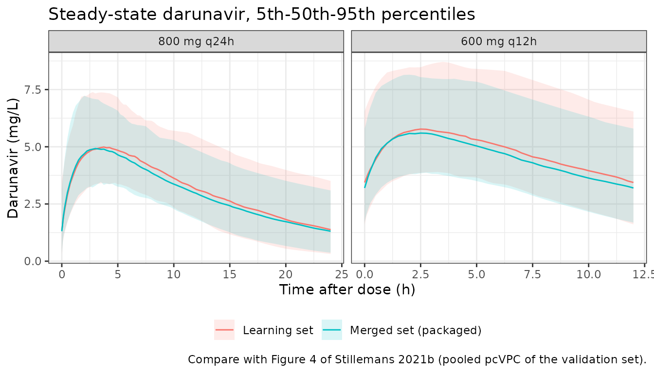
PKNCA validation
nca_input <- sim_merged |>
  filter(!is.na(Cc)) |>
  mutate(tad = time - 14 * 24) |>
  filter(tad >= 0) |>
  select(id, regimen, tad, Cc)

dose_df <- regimens |>
  tidyr::crossing(subject = seq_len(n_subj)) |>
  mutate(
    id = (match(regimen, regimens$regimen) - 1L) * n_subj + subject,
    tad = 0
  ) |>
  select(id, regimen, tad, dose, tau)

conc_obj <- PKNCA::PKNCAconc(nca_input, Cc ~ tad | regimen + id,
  concu = "mg/L", timeu = "h"
)
dose_obj <- PKNCA::PKNCAdose(dose_df, dose ~ tad | regimen + id,
  doseu = "mg"
)
intervals <- regimens |>
  transmute(
    regimen,
    start = 0, end = tau,
    auclast = TRUE, cmax = TRUE, tmax = TRUE, cmin = TRUE
  ) |>
  as.data.frame()
nca_res <- PKNCA::pk.nca(PKNCA::PKNCAdata(conc_obj, dose_obj, intervals = intervals))
nca <- as.data.frame(nca_res)

nca_wide <- nca |>
  select(id, regimen, PPTESTCD, PPORRES) |>
  tidyr::pivot_wider(names_from = PPTESTCD, values_from = PPORRES) |>
  left_join(cl_ind |> select(id, cl), by = "id") |>
  left_join(regimens, by = "regimen") |>
  mutate(auc_theory = dose / cl, pct_diff = 100 * (auclast / auc_theory - 1))

# At steady state AUC over one interval equals Dose / CL for each patient.
# Both sides use the same drawn parameters, so the difference is only the
# trapezoidal error of the 0.25-h grid.
stopifnot(all(abs(nca_wide$pct_diff) < 1))

nca_wide |>
  group_by(regimen) |>
  summarise(
    auc_median = median(auclast),
    auc_p025 = quantile(auclast, 0.025),
    auc_p975 = quantile(auclast, 0.975),
    cmax_median = median(cmax),
    cmin_median = median(cmin),
    tmax_median = median(tmax),
    .groups = "drop"
  ) |>
  dplyr::rename(
    "Regimen" = regimen,
    "AUCtau median (mg*h/L)" = auc_median,
    "AUCtau 2.5th pct" = auc_p025,
    "AUCtau 97.5th pct" = auc_p975,
    "Cmax median (mg/L)" = cmax_median,
    "Ctrough median (mg/L)" = cmin_median,
    "Tmax median (h)" = tmax_median
  ) |>
knitr::kable(digits = 2, caption = "Steady-state NCA of the merged-set model (virtual validation-design cohort).")| Regimen | AUCtau median (mg*h/L) | AUCtau 2.5th pct | AUCtau 97.5th pct | Cmax median (mg/L) | Ctrough median (mg/L) | Tmax median (h) |
|---|---|---|---|---|---|---|
| 600 mg q12h | 54.58 | 32.43 | 94.80 | 5.68 | 3.20 | 2.75 |
| 800 mg q24h | 72.77 | 43.24 | 126.41 | 5.08 | 1.31 | 3.25 |
Comparison with the published AUC range
The paper prints no NCA table. It does give “a clinically meaningful range of 50 to 130 mg h l-1”, described as the 95% prediction interval of the 24-hour AUC in the learning set. That interval came from the full model with AAG, simulated from the learning-set patients’ own covariates. Most of those patients took 800 mg once daily. The comparison below uses the 800 mg once-daily arm of the merged-set model. The reduced model has no AAG variability, and its cohort uses the validation set’s covariate frequencies. Close agreement is therefore expected only for the centre of the interval, not its tails.
auc_800 <- nca_wide |> filter(regimen == "800 mg q24h")
auc_cmp <- tibble::tibble(
  Statistic = c("2.5th percentile", "Median", "97.5th percentile"),
  Simulated = unname(quantile(auc_800$auclast, c(0.025, 0.5, 0.975))),
  Published = c(50, NA, 130)
)
knitr::kable(auc_cmp, digits = 1, caption = "AUC0-24 at 800 mg once daily versus the paper's 95% prediction interval (mg*h/L).")| Statistic | Simulated | Published |
|---|---|---|
| 2.5th percentile | 43.2 | 50 |
| Median | 72.8 | NA |
| 97.5th percentile | 126.4 | 130 |
# The typical 800-mg AUC for the reference patient is Dose / CL = 64.5.
# The cohort median must sit inside the published interval. Both simulated
# tails must fall within 30% of the published limits: the tails of a
# 200-patient cohort are not a precise statistic, and the published interval
# includes AAG variability that this model does not have.
stopifnot(
  auc_cmp$Simulated[2] > 50, auc_cmp$Simulated[2] < 130,
  abs(auc_cmp$Simulated[1] / 50 - 1) < 0.3,
  abs(auc_cmp$Simulated[3] / 130 - 1) < 0.3
)
Optimal sampling strategies (not reproduced)
Table 3 evaluates one- to three-point sampling strategies by maximum a posteriori Bayesian estimation of each simulated patient’s clearance. The simulations used the learning-set patients with their baseline covariates and the final NONMEM model. The paper also notes that “the validation set could not be used due to the lack of AAG”, which points to the full model. That evaluation needs individual AAG values and a Bayesian re-estimation step, and neither can be reproduced from the published information. It is therefore not repeated here. The recommended designs were C1-C4-C19 (D-optimal) and C0-C1-C4 (near-optimal; RMSPE of AUC 12.0% and 12.8%).
Assumptions and deviations
-
Parameter set. The packaged model uses the
merged-set re-estimate (Table 2). That is the paper’s final estimate of
the validated reduced model. The learning-set estimates are applied
above through
rxode2::ini(). The full model with AAG belongs to the companion paper (Stillemans 2021, Clin Pharmacokinet) and is not part of this model. - Equation forms. This paper does not restate the covariate equations. The forms (exponential for sex; categorical for CYP3A5*3 and SLCO3A1) are those of the underlying model, from its ESM Online Resource 2. The sign of the CYP3A5 coefficient (-0.126, applied to *3/*3 nonexpressers) follows that model’s parameterisation (‘CYP3A5*3 on CL’).
- Residual error. The ‘exponential’ residual error is encoded as proportional, together with the additive term (combined error, SDs as printed).
- Separate occasions. The merged fit treated the 51 patients in both studies as separate occasions, and the paper prints no between-occasion variability. The packaged model has between-subject variability only.
- No PRIOR. The learning-set model was estimated with a NONMEM PRIOR on the fixed and random effects. The packaged values are the posterior estimates the paper reports.
- Booster. Booster (cobicistat vs ritonavir) is not a covariate. The external validation found the model adequate for ritonavir-boosted patients although it was developed mostly on cobicistat data.
- Virtual cohort. Missing genotypes are ignored when setting the cohort frequencies; the paper imputed the most frequent genotype for each patient’s race.