Brazikumab PK and biomarker-driven CDAI response (Zhang 2023) • nlmixr2lib

Model and source

Zhang 2023 is a single paper that reports three models, so nlmixr2lib ships it as three model files that share this one vignette:

Model	Role
`Zhang_2023_brazikumab`	Final population PK model (phase Ib + phase IIa, all PK data)
`Zhang_2023_brazikumab_il22`	CDAI indirect-response PK/PD model with a baseline IL-22-dependent drug effect
`Zhang_2023_brazikumab_crp`	CDAI indirect-response PK/PD model with a baseline CRP-dependent drug effect

The two efficacy models are alternatives, not a joint fit: the authors report that adding both biomarkers together “did not result in a more statistically significant relationship … possibly due to the small sample size of the treatment arm and that BIL22 and BCRP are 60% correlated”.

Citation: Zhang N, Chan ML, Li J, Brohawn PZ, Sun B, Vainshtein I, Roskos LK, Faggioni R, Savic RM. Combining pharmacometric models with predictive and prognostic biomarkers for precision therapy in Crohn’s disease: A case study of brazikumab. CPT Pharmacometrics Syst Pharmacol. 2023;12(12):1945-1959. doi:10.1002/psp4.13044
Article: https://doi.org/10.1002/psp4.13044
Supplement (Appendix S1 + NONMEM control streams + analysis dataset): https://doi.org/10.1002/psp4.13044

mod_pk   <- rxode2::rxode2(readModelDb("Zhang_2023_brazikumab"))
#> ℹ parameter labels from comments will be replaced by 'label()'
mod_il22 <- rxode2::rxode2(readModelDb("Zhang_2023_brazikumab_il22"))
#> ℹ parameter labels from comments will be replaced by 'label()'
mod_crp  <- rxode2::rxode2(readModelDb("Zhang_2023_brazikumab_crp"))
#> ℹ parameter labels from comments will be replaced by 'label()'

Brazikumab (MEDI2070 / AMG139) is a human IgG monoclonal antibody against the p19 subunit of interleukin-23 (IL-23), developed for Crohn’s disease (CD) and ulcerative colitis. IL-23 drives downstream IL-22 production, which is elevated in CD and tracks disease activity – the mechanistic reason the authors chose an indirect-response model with inhibition of the CDAI production rate (kin) rather than stimulation of its elimination rate (kout).

Population

The population PK model pooled all PK data from two trials: a phase Ib multiple-ascending-dose study (NCT01258205, n = 34: 30 healthy participants and 4 patients with CD; 70-700 mg IV or 210 mg SC Q4W; median 21 PK samples per subject) and a phase IIa study (NCT01714726, n = 119 patients with moderately to severely active CD who had failed or were intolerant to anti-TNF-alpha therapy; median 9 PK samples per subject), including the phase IIa open-label period.

The biomarker/efficacy models used only the 12-week double-blind placebo-controlled induction period of the phase IIa trial (59 brazikumab, 60 placebo). The authors excluded the 100-week open-label period “due to potential influence of unblinding on the clinical readout”. Median baseline values in the phase IIa cohort were CDAI 317, IL-22 15.6 pg/mL, and CRP 15.7 mg/L; the cohort was 62% female, 93% White, median age 35 years and median weight 66.9 kg (Table 1).

The same information is available programmatically via each model’s population metadata (readModelDb("Zhang_2023_brazikumab")()$population).

readModelDb("Zhang_2023_brazikumab_il22")()$population$baseline_covariates |>
  tibble::enframe(name = "Baseline characteristic", value = "Value") |>
  mutate(Value = unlist(Value)) |>
  knitr::kable(caption = "Phase IIa baseline characteristics carried in the model metadata (Zhang 2023 Table 1).")

Phase IIa baseline characteristics carried in the model metadata (Zhang 2023 Table 1).
Baseline characteristic	Value
cdai_median_all	317.0
cdai_median_treatment	330.0
cdai_median_placebo	304.0
il22_median_all_pg_mL	15.6
il22_median_treatment	15.9
il22_median_placebo	14.1
crp_median_all_mg_L	15.7
albumin_median_g_L	39.0

Source trace

Every ini() entry in the three model files carries an in-file comment naming its source location. They are collected here for review.

Equation / parameter	Value	Source location
Population PK model (`Zhang_2023_brazikumab`)
`lcl` (CL)	0.26 L/day	Table 2, “CL in female patients with CD” (RSE 5%)
`lvc` (Vc)	3.27 L	Table 2, “Vc in female subjects” (RSE 5%)
`lvp` (Vp)	2.64 L	Table 2, “Vp” (RSE 8%)
`lq` (Q)	0.412 L/day	Table 2, “Q” (RSE 19%)
`lka` (ka)	0.286 1/day	Table 2, “ka” (RSE 11%)
`ltlag` (Tlag)	0.0296 day	Table 2, “Tlag” (RSE 14%)
`lfdepot` (F)	0.88	Table 2, “F” (RSE 5%)
`e_alb_cl`	-1.32	Table 2, “Effect of baseline albumin on CL” (RSE 40%); footnote a
`e_dis_healthy_cl`	-0.362	Table 2, “Effect of health status on CL” (RSE 10%); footnote a
`e_male_vc`	0.214	Table 2, “Effect of male gender on Vc” (RSE 37%); footnote b
`etalcl`	0.131	Table 2, IIV column for CL (RSE 33%)
`etalvc`	0.0502	Table 2, IIV column for Vc (RSE 18%)
`propSd`	0.249	Table 2, “Proportional error” 24.9% (RSE 9%)
ODEs `depot` / `central` / `peripheral1`	n/a	Appendix S1 Equations 1-6
CL / Vc covariate equations	n/a	Table 2 footnotes a and b
IL-22 efficacy model (`Zhang_2023_brazikumab_il22`)
`lrbase` (baseline CDAI)	318	Table 2, IL-22 column, “Baseline CDAI” (RSE 3%)
`lthalfrec` (HL)	11.6 day	Table 2, IL-22 column, “Half-life HL” (RSE 33%)
`iplac`	0.209	Table 2, IL-22 column, “Inhibitory placebo effect” (RSE 7%)
`limax` (Imax)	0.297	Table 2, IL-22 column, “Imax” (RSE 30%)
`lec50` (the paper’s IB50)	22.8 pg/mL	Table 2, IL-22 column, “IB50” (RSE 10%)
`hill` (the paper’s gamma)	20 FIXED	Table 2, IL-22 column, “Hill coefficient gamma = 20 FIX”
`etalrbase`	0.0106	Table 2, IL-22 column, “IIV of BCDAI score” (RSE 74%)
`etaiplac`	0.0509	Table 2, IL-22 column, “IIV of placebo effect” (RSE 26%)
`etalrbase`/`etaiplac` correlation	-100% (encoded -99%)	Table 2, IL-22 column, “Correlation between IIV of BCDAI score and placebo effect”
`propSd_cdai`	0.116	Table 2, IL-22 column, “Proportional error, efficacy” (RSE 42%)
`addSd_cdai`	38.9	Table 2, IL-22 column, “Additive error, efficacy” (RSE 28%)
CRP efficacy model (`Zhang_2023_brazikumab_crp`)
`lrbase` (baseline CDAI)	318	Table 2, CRP column (RSE 2%)
`lthalfrec` (HL)	11.7 day	Table 2, CRP column (RSE 8%)
`iplac`	0.178	Table 2, CRP column (RSE 16%)
`limax` (Imax)	0.246	Table 2, CRP column (RSE 10%)
`lec50` (the paper’s IB50)	8.03 mg/L	Table 2, CRP column (RSE 10%)
`hill` (the paper’s gamma)	2.07 FIXED	Table 2, CRP column, “Hill coefficient gamma = 2.07 FIX”
`etalrbase`	0.00997	Table 2, CRP column (RSE 35%)
`etaiplac`	0.0519	Table 2, CRP column (RSE 4%)
`propSd_cdai` / `addSd_cdai`	0.117 / 38.9	Table 2, CRP column (RSE 9% / 8%)
IDR equations `kin`, `kout`, `Itotal`	n/a	Equations 1-4 (page 1949)
Biomarker sigmoid `Imax * CB^g / (IB50^g + CB^g)`	n/a	Equation 5 (page 1950); Figure 2
Drug effect zero in placebo arm	n/a	Supplement control streams s04.mod / s05.mod: `EFF = 0; IF(ARM.EQ.1) EFF = ...`
PK parameters held FIXED in efficacy fits	n/a	s04.mod / s05.mod `$THETA` rows 1-13 all carry `FIX`

Virtual cohort

Original participant-level data are not redistributable, so the figures below use virtual populations whose covariate distributions approximate the published trial demographics (Table 1). Cohorts are 100 subjects per arm.

Baseline IL-22 and CRP are strongly right-skewed in the source cohort (IL-22 median 15.9 pg/mL with a maximum of 711; CRP median 18.2 mg/L with a maximum of 212.8), so both are drawn from log-normal distributions calibrated to the published median and approximate range and then clipped to the observed limits.

set.seed(20231206)
n_arm <- 100L

# Log-normal calibrated to a target median and 97.5th percentile, then clipped
# to the published observed range.
rlnorm_median <- function(n, med, p975, lo, hi) {
  sdlog <- log(p975 / med) / qnorm(0.975)
  pmin(pmax(rlnorm(n, meanlog = log(med), sdlog = sdlog), lo), hi)
}

make_efficacy_arm <- function(n, on_treatment, arm_label, id_offset,
                              il22_med, crp_med) {
  subj <- tibble(
    id           = id_offset + seq_len(n),
    arm          = arm_label,
    ON_TREATMENT = as.integer(on_treatment),
    DIS_HEALTHY  = 0L,
    SEXF         = rbinom(n, 1L, 0.622),
    ALB          = pmin(pmax(rnorm(n, 39, 3.5), 32), 50),
    IL22         = rlnorm_median(n, il22_med, 170, 1.00, 711),
    CRP          = rlnorm_median(n, crp_med, 110, 0.32, 212.8)
  )
  # Phase IIa induction: 700 mg IV over 1 h on day 1 and day 29 (placebo arm gets
  # the same schedule; ON_TREATMENT = 0 switches the drug effect off).
  doses <- subj |>
    tidyr::crossing(tibble(time = c(0, 28))) |>
    mutate(amt = 700, evid = 1L, cmt = "central", rate = 700 / (1 / 24))
  # Observation rows must sit on an ENDPOINT compartment for this two-endpoint
  # model: "Cc" for concentration, "cdai" for the CDAI score.
  obs <- subj |>
    tidyr::crossing(tibble(time = seq(0, 84, by = 3.5))) |>
    tidyr::crossing(tibble(cmt = c("Cc", "cdai"))) |>
    mutate(amt = NA_real_, evid = 0L, rate = NA_real_)
  bind_rows(doses, obs) |> arrange(id, time, desc(evid))
}

ev_eff <- bind_rows(
  make_efficacy_arm(n_arm, TRUE,  "Brazikumab 700 mg IV", 0L,     15.9, 18.2),
  make_efficacy_arm(n_arm, FALSE, "Placebo",              1000L,  14.1, 9.55)
)
stopifnot(!anyDuplicated(unique(ev_eff[, c("id", "time", "evid", "cmt")])))

The phase Ib / IIa PK cohorts reproduce the dose groups of Figure 1a: healthy participants at 70, 210, 420, and 700 mg IV and 210 mg SC, plus patients with CD at 700 mg IV, all Q4W for three doses.

make_pk_cohort <- function(n, dose, route, dis_healthy, label, id_offset) {
  subj <- tibble(
    id          = id_offset + seq_len(n),
    cohort      = label,
    DIS_HEALTHY = as.integer(dis_healthy),
    SEXF        = rbinom(n, 1L, if (dis_healthy) 0.118 else 0.622),
    ALB         = pmin(pmax(rnorm(n, 39, 3.5), 32), 50)
  )
  doses <- subj |>
    tidyr::crossing(tibble(time = c(0, 28, 56))) |>
    mutate(amt = dose, evid = 1L,
           cmt  = if (route == "IV") "central" else "depot",
           rate = if (route == "IV") dose / (1 / 24) else 0)
  obs <- subj |>
    tidyr::crossing(tibble(time = seq(0, 112, by = 3.5))) |>
    mutate(amt = NA_real_, evid = 0L, cmt = "central", rate = NA_real_)
  bind_rows(doses, obs) |> arrange(id, time, desc(evid))
}

pk_groups <- tibble::tribble(
  ~dose, ~route, ~dis_healthy, ~label,
  70,    "IV",   TRUE,         "HV 70 mg IV",
  210,   "IV",   TRUE,         "HV 210 mg IV",
  420,   "IV",   TRUE,         "HV 420 mg IV",
  700,   "IV",   TRUE,         "HV 700 mg IV",
  210,   "SC",   TRUE,         "HV 210 mg SC",
  700,   "IV",   FALSE,        "CD 700 mg IV"
)

ev_pk <- do.call(bind_rows, lapply(seq_len(nrow(pk_groups)), function(i) {
  make_pk_cohort(50L, pk_groups$dose[i], pk_groups$route[i],
                 pk_groups$dis_healthy[i], pk_groups$label[i],
                 id_offset = (i - 1L) * 100L)
}))
stopifnot(!anyDuplicated(unique(ev_pk[, c("id", "time", "evid")])))

Population PK

sim_pk <- rxode2::rxSolve(
  mod_pk, events = ev_pk, keep = c("cohort"),
  useLinCmt = FALSE   # rxode2's ODE->linCmt auto-conversion is bypassed for consistency with the PK/PD models
) |> as.data.frame()

# Replicates Figure 1a of Zhang 2023: PK profiles stratified by population and route.
sim_pk |>
  filter(time > 0) |>
  group_by(cohort, time) |>
  summarise(Q05 = quantile(Cc, 0.05), Q50 = median(Cc), Q95 = quantile(Cc, 0.95),
            .groups = "drop") |>
  ggplot(aes(time, Q50)) +
  geom_ribbon(aes(ymin = Q05, ymax = Q95), alpha = 0.2) +
  geom_line(linewidth = 0.6) +
  facet_wrap(~cohort) +
  scale_y_log10() +
  labs(x = "Time (day)", y = "Brazikumab concentration (ug/mL)",
       title = "Figure 1a -- PK by population and route (Q4W x 3 doses)",
       caption = "Replicates Figure 1a of Zhang 2023. Ribbon = 5th-95th percentile.")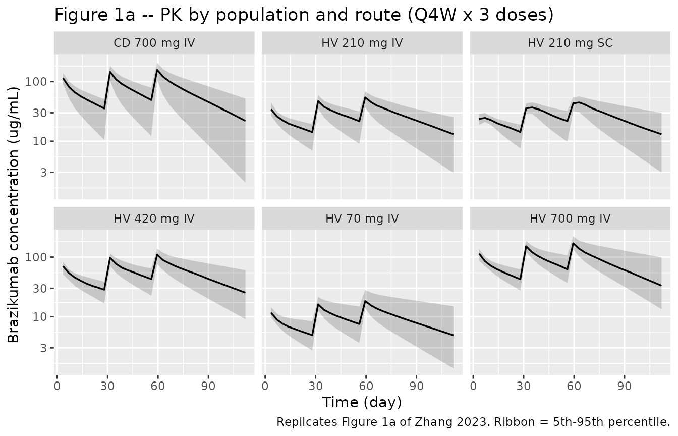

The paper’s two headline covariate findings are recovered exactly. Healthy participants clear brazikumab 36.2% more slowly than patients with CD at the same baseline albumin, and a 10% rise in albumin lowers CL by 11.8% (1.1^-1.32 = 0.882).

# Typical-value check: with the random effects switched off and albumin at the
# reference 39 g/L, the model must return the Table 2 typical CL exactly.
cl_typical <- local({
  subj <- tibble(id = 1:2, DIS_HEALTHY = c(0L, 1L), SEXF = 1L, ALB = 39)
  ev <- bind_rows(
    subj |> mutate(time = 0, amt = 700, evid = 1L, cmt = "central", rate = 700 / (1 / 24)),
    subj |> mutate(time = 7, amt = NA_real_, evid = 0L, cmt = "central", rate = NA_real_)
  ) |> arrange(id, time, desc(evid))
  rxode2::rxSolve(mod_pk, events = ev, omega = NA, useLinCmt = FALSE) |>
    as.data.frame() |>
    transmute(Cohort = ifelse(DIS_HEALTHY == 1, "Healthy participant", "Patient with CD"),
              `Typical CL (L/day)` = signif(cl, 4))
})
#> Warning: multi-subject simulation without without 'omega'

cl_typical |>
  mutate(`Published (Table 2)` = signif(c(0.26, 0.26 * (1 - 0.362)), 4),
         `Difference (%)` = round(100 * (`Typical CL (L/day)` - `Published (Table 2)`) /
                                    `Published (Table 2)`, 2)) |>
  knitr::kable(caption = "Typical CL at the reference covariates (albumin 39 g/L, random effects zeroed) vs. the Zhang 2023 Table 2 values.")

Typical CL at the reference covariates (albumin 39 g/L, random effects zeroed) vs. the Zhang 2023 Table 2 values.
Cohort	Typical CL (L/day)	Published (Table 2)	Difference (%)
Patient with CD	0.2600	0.2600	0
Healthy participant	0.1659	0.1659	0


sim_pk |>
  filter(time > 56, cohort %in% c("HV 700 mg IV", "CD 700 mg IV")) |>
  group_by(cohort, time) |>
  summarise(Q50 = median(Cc), .groups = "drop") |>
  ggplot(aes(time, Q50, colour = cohort)) +
  geom_line(linewidth = 0.8) +
  scale_y_log10() +
  labs(x = "Time (day)", y = "Brazikumab concentration (ug/mL)", colour = NULL,
       title = "Figure 1b -- elimination phase after the third 700 mg IV dose",
       caption = "Replicates Figure 1b of Zhang 2023: HVs eliminate brazikumab more slowly than patients with CD.")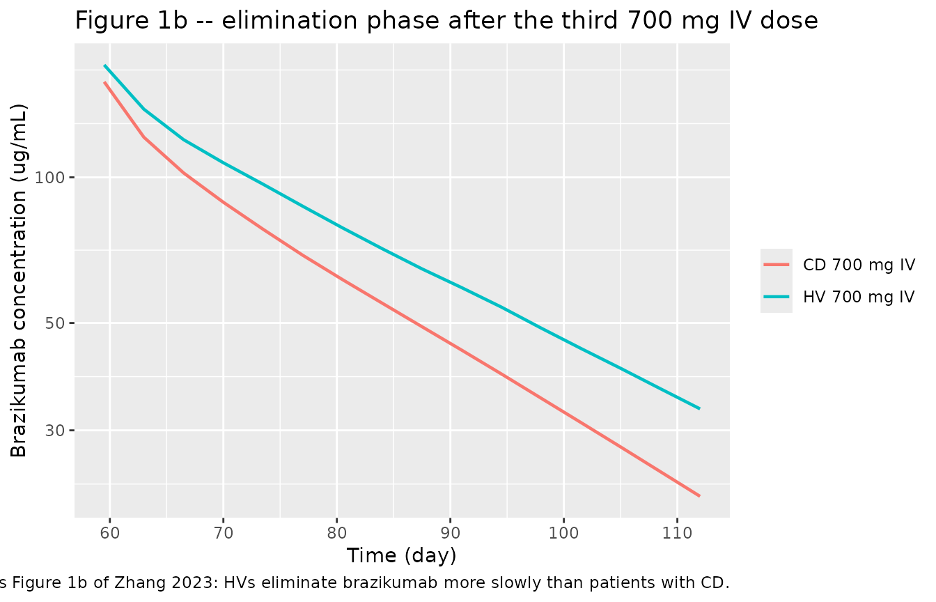

PKNCA validation

NCA is run on the phase IIa induction regimen (700 mg IV on day 1 and day 29, followed to day 84) because that is the exposure the paper characterises numerically. A daily observation grid is used so the trapezoidal AUC resolves the post-infusion peak.

ev_iia <- local({
  subj <- tibble(
    id     = seq_len(100L),
    cohort = "CD 700 mg IV q4w",
    DIS_HEALTHY = 0L,
    SEXF   = rbinom(100L, 1L, 0.622),
    ALB    = pmin(pmax(rnorm(100L, 39, 3.5), 32), 50)
  )
  bind_rows(
    subj |> tidyr::crossing(tibble(time = c(0, 28))) |>
      mutate(amt = 700, evid = 1L, cmt = "central", rate = 700 / (1 / 24)),
    subj |> tidyr::crossing(tibble(time = seq(0, 84, by = 1))) |>
      mutate(amt = NA_real_, evid = 0L, cmt = "central", rate = NA_real_)
  ) |> arrange(id, time, desc(evid))
})

sim_iia <- rxode2::rxSolve(mod_pk, events = ev_iia, keep = c("cohort"),
                           useLinCmt = FALSE) |> as.data.frame()

sim_nca <- sim_iia |>
  dplyr::filter(!is.na(Cc)) |>
  dplyr::select(id, time, Cc, cohort)

# Guarantee a time-zero row per subject (IV pre-dose Cc = 0) so PKNCA can anchor
# the AUC interval; without it PKNCA warns once per subject.
sim_nca <- bind_rows(
  sim_nca,
  sim_nca |> distinct(id, cohort) |> mutate(time = 0, Cc = 0)
) |>
  distinct(id, cohort, time, .keep_all = TRUE) |>
  arrange(id, cohort, time)

conc_obj <- PKNCA::PKNCAconc(sim_nca, Cc ~ time | cohort + id)

dose_df <- ev_iia |>
  filter(evid == 1) |>
  select(id, time, amt, cohort) |>
  mutate(duration = 1 / 24)   # 1 h IV infusion; PKNCAdose needs it for Vss

dose_obj <- PKNCA::PKNCAdose(dose_df, amt ~ time | cohort + id, duration = "duration")

# Two intervals: 0-56 days (through week 8, the window the paper's average-exposure
# figure uses) and 0-84 days (the full double-blind period).
intervals <- data.frame(
  start     = c(0,     0),
  end       = c(56,    84),
  cav       = c(TRUE,  TRUE),
  cmax      = c(FALSE, TRUE),
  tmax      = c(FALSE, TRUE),
  auclast   = c(FALSE, TRUE),
  half.life = c(FALSE, TRUE)
)

nca_res <- PKNCA::pk.nca(PKNCA::PKNCAdata(conc_obj, dose_obj, intervals = intervals))

nca_summary <- as.data.frame(nca_res) |>
  filter(PPTESTCD %in% c("cmax", "tmax", "auclast", "cav", "half.life")) |>
  group_by(PPTESTCD, start, end) |>
  summarise(P05 = quantile(PPORRES, 0.05, na.rm = TRUE),
            P50 = median(PPORRES, na.rm = TRUE),
            P95 = quantile(PPORRES, 0.95, na.rm = TRUE), .groups = "drop") |>
  mutate(across(c(P05, P50, P95), \(x) signif(x, 3))) |>
  arrange(end, PPTESTCD)

nca_summary |>
  mutate(Interval = paste0(start, "-", end, " day")) |>
  select(-start, -end) |>
  relocate(Interval, .after = PPTESTCD) |>
  rename("NCA parameter" = PPTESTCD, "5th pctile" = P05,
         "Median" = P50, "95th pctile" = P95) |>
  knitr::kable(caption = paste("Simulated NCA for the phase IIa induction regimen",
                               "(700 mg IV on days 1 and 29). Units: cmax / cav in ug/mL,",
                               "auclast in ug*day/mL, tmax and half.life in day."))

Simulated NCA for the phase IIa induction regimen (700 mg IV on days 1 and 29). Units: cmax / cav in ug/mL, auclast in ug*day/mL, tmax and half.life in day.
NCA parameter	Interval	5th pctile	Median	95th pctile
auclast	0-56 day	2520.0	3900.0	5450.0
cav	0-56 day	45.0	69.7	97.3
auclast	0-84 day	2690.0	4510.0	7060.0
cav	0-84 day	32.0	53.7	84.0
cmax	0-84 day	151.0	191.0	243.0
half.life	0-84 day	11.4	18.3	31.6
tmax	0-84 day	29.0	29.0	29.0

Zhang 2023 does not publish an NCA table, so there is no full side-by-side comparison to make. The one exposure metric the paper does quantify is the spread of average brazikumab concentration in the phase IIa treatment arm: “the 5th and 95th percentiles of the average exposures: 43.7-106.1 ug/mL” (Results). That maps directly onto PKNCA’s cav. The paper introduces this range while discussing Figure S1, which relates each patient’s average concentration to their week-8 CDAI change, so the 0-56 day interval is the matching window; the 0-84 day average is lower because no dose is given after day 29 and the last four weeks are pure washout.

cav_tab <- as.data.frame(nca_res) |>
  filter(PPTESTCD == "cav") |>
  group_by(end) |>
  summarise(P05 = quantile(PPORRES, 0.05, na.rm = TRUE),
            P95 = quantile(PPORRES, 0.95, na.rm = TRUE), .groups = "drop")

bind_rows(
  tibble::tibble(
    Interval   = "0-56 day (through week 8)",
    Percentile = c("5th", "95th"),
    Simulated  = signif(c(cav_tab$P05[cav_tab$end == 56], cav_tab$P95[cav_tab$end == 56]), 3),
    Published  = c(43.7, 106.1)
  ),
  tibble::tibble(
    Interval   = "0-84 day (full double-blind period)",
    Percentile = c("5th", "95th"),
    Simulated  = signif(c(cav_tab$P05[cav_tab$end == 84], cav_tab$P95[cav_tab$end == 84]), 3),
    Published  = c(43.7, 106.1)
  )
) |>
  mutate(`Difference (%)` = round(100 * (Simulated - Published) / Published, 1)) |>
  knitr::kable(caption = "Average brazikumab concentration (Cav, ug/mL) vs. the published 5th-95th percentile range (Zhang 2023 Results). The 0-56 day row is the like-for-like comparison; the 0-84 day row is shown for context.")

Average brazikumab concentration (Cav, ug/mL) vs. the published 5th-95th percentile range (Zhang 2023 Results). The 0-56 day row is the like-for-like comparison; the 0-84 day row is shown for context.
Interval	Percentile	Simulated	Published	Difference (%)
0-56 day (through week 8)	5th	45.0	43.7	3.0
0-56 day (through week 8)	95th	97.3	106.1	-8.3
0-84 day (full double-blind period)	5th	32.0	43.7	-26.8
0-84 day (full double-blind period)	95th	84.0	106.1	-20.8

Biomarker-driven CDAI response

sim_il22 <- rxode2::rxSolve(mod_il22, events = ev_eff, keep = c("arm"),
                            useLinCmt = FALSE) |> as.data.frame()
sim_crp  <- rxode2::rxSolve(mod_crp,  events = ev_eff, keep = c("arm"),
                            useLinCmt = FALSE) |> as.data.frame()

# rxSolve returns observation rows only. Both endpoints observe at each time, so
# each (id, time) appears twice; collapse to one row per (id, time) for plotting --
# rxSolve returns every model variable (including both `Cc` and `cdai`) on every
# row regardless of which endpoint that row points at.
collapse_rows <- function(x) {
  x |> distinct(id, time, .keep_all = TRUE)
}
sim_il22_1 <- collapse_rows(sim_il22)
sim_crp_1  <- collapse_rows(sim_crp)

# Replicates Figure 1c of Zhang 2023: CDAI over the double-blind period by arm.
sim_il22_1 |>
  group_by(arm, time) |>
  summarise(Q05 = quantile(cdai, 0.05), Q50 = median(cdai),
            Q95 = quantile(cdai, 0.95), .groups = "drop") |>
  ggplot(aes(time, Q50, colour = arm, fill = arm)) +
  geom_ribbon(aes(ymin = Q05, ymax = Q95), alpha = 0.18, colour = NA) +
  geom_line(linewidth = 0.8) +
  labs(x = "Time (day)", y = "CDAI score", colour = NULL, fill = NULL,
       title = "Figure 1c -- CDAI over the 12-week double-blind period (IL-22 model)",
       caption = "Replicates Figure 1c of Zhang 2023. Ribbon = 5th-95th percentile.")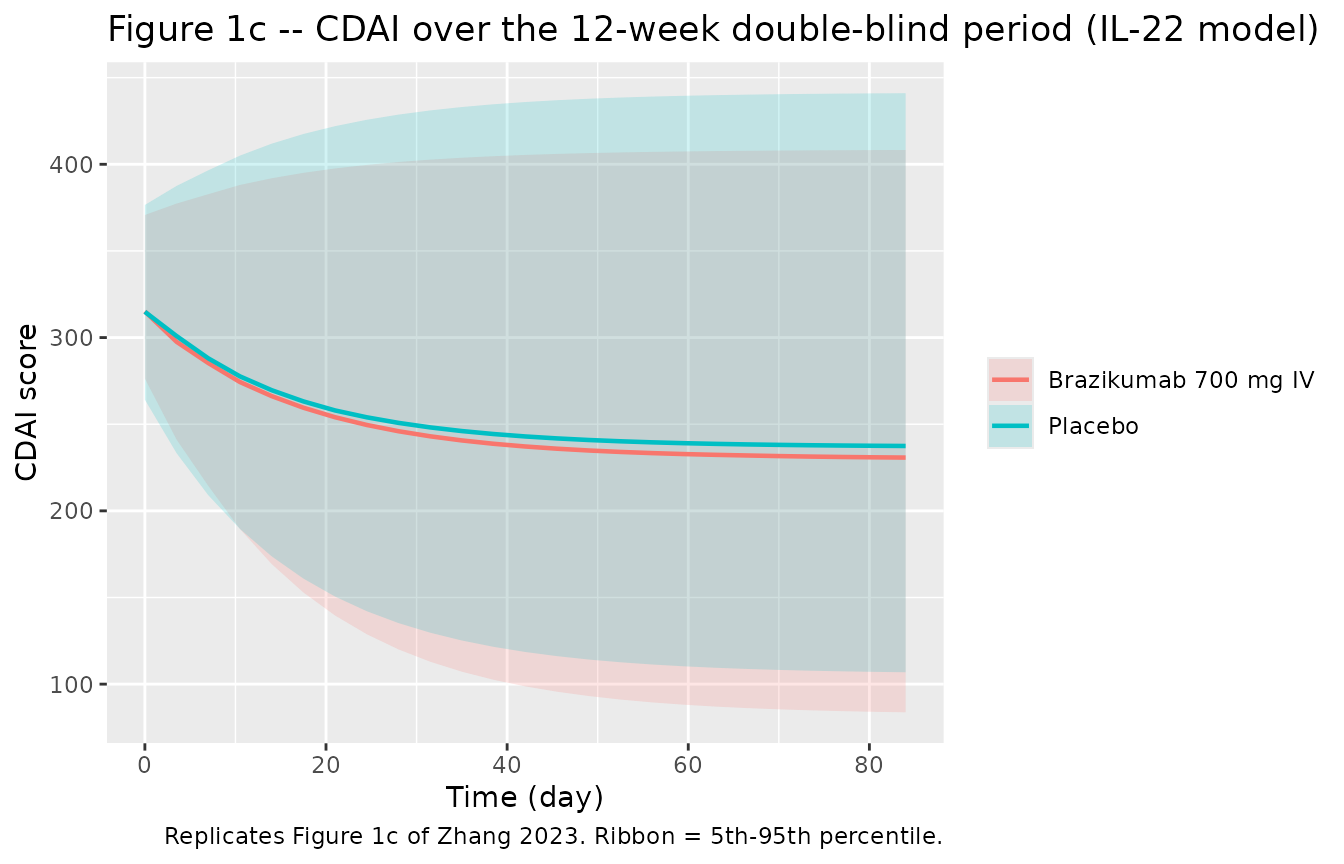

Total inhibition as a function of the baseline biomarker

Figure 4 of the paper plots the total inhibition of the CDAI input rate against the baseline biomarker level: a flat placebo-only line and a rising total-effect curve. Rather than re-implementing Equation 5, the curves below are read straight out of the packaged models by solving them across a grid of baseline biomarker values with the random effects switched off.

itotal_curve <- function(mod, biomarker, grid, label) {
  subj <- tibble(id = seq_along(grid), DIS_HEALTHY = 0L, SEXF = 1L, ALB = 39,
                 ON_TREATMENT = 1L, IL22 = 15.9, CRP = 18.2)
  subj[[biomarker]] <- grid
  ev <- bind_rows(
    subj |> mutate(time = 0, amt = 700, evid = 1L, cmt = "central", rate = 700 / (1 / 24)),
    subj |> mutate(time = 0, amt = NA_real_, evid = 0L, cmt = "cdai", rate = NA_real_)
  ) |> arrange(id, time, desc(evid))
  rxode2::rxSolve(mod, events = ev, omega = NA, useLinCmt = FALSE) |>
    as.data.frame() |>
    distinct(id, time, .keep_all = TRUE) |>
    transmute(model = label, biomarker_level = grid[id],
              placebo_only = iplac_i, total = itotal)
}

grid_il22 <- exp(seq(log(1), log(711), length.out = 60))
grid_crp  <- exp(seq(log(0.32), log(212.8), length.out = 60))

curves <- bind_rows(
  itotal_curve(mod_il22, "IL22", grid_il22, "a) Baseline IL-22 (pg/mL)"),
  itotal_curve(mod_crp,  "CRP",  grid_crp,  "b) Baseline CRP (mg/L)")
)
#> Warning: multi-subject simulation without without 'omega'
#> Warning: multi-subject simulation without without 'omega'

curves |>
  tidyr::pivot_longer(c(placebo_only, total), names_to = "component", values_to = "inhibition") |>
  mutate(component = recode(component,
                            placebo_only = "Placebo effect only",
                            total = "Total (placebo + drug)")) |>
  ggplot(aes(biomarker_level, 100 * inhibition, colour = component)) +
  geom_line(linewidth = 0.9) +
  facet_wrap(~model, scales = "free_x") +
  scale_x_log10() +
  labs(x = "Baseline biomarker level (log scale)",
       y = "Inhibition of the CDAI input rate (%)", colour = NULL,
       title = "Figure 4 -- biomarker-dependent inhibition of the CDAI input rate",
       caption = "Replicates Figure 4a/4b of Zhang 2023.")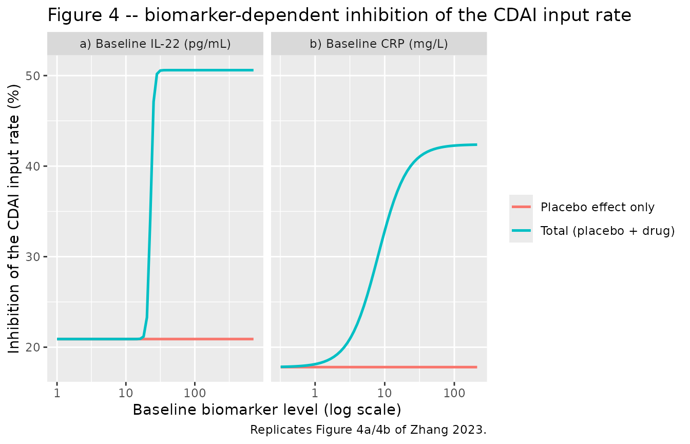

The plateau values are the paper’s headline result and are reproduced exactly, because they are just iplac and iplac + Imax:

anchor <- function(mod_name, lab, lo_pub, hi_pub) {
  p <- readModelDb(mod_name)() |> rxode2::rxode2()
  th <- p$theta
  lo <- unname(th[["iplac"]])
  hi <- lo + exp(unname(th[["limax"]]))
  tibble(Model = lab,
         `Low biomarker, simulated (%)`  = round(100 * lo, 1),
         `Low biomarker, published (%)`  = lo_pub,
         `High biomarker, simulated (%)` = round(100 * hi, 1),
         `High biomarker, published (%)` = hi_pub)
}

bind_rows(
  anchor("Zhang_2023_brazikumab_il22", "IL-22 model", 20.9, 50.6),
  anchor("Zhang_2023_brazikumab_crp",  "CRP model",   17.8, 42.4)
) |>
  knitr::kable(caption = "Maximal total inhibition of the CDAI input rate at extreme biomarker levels, vs. the values reported in the Zhang 2023 Abstract and Results.")

Maximal total inhibition of the CDAI input rate at extreme biomarker levels, vs. the values reported in the Zhang 2023 Abstract and Results.
Model	Low biomarker, simulated (%)	Low biomarker, published (%)	High biomarker, simulated (%)	High biomarker, published (%)
IL-22 model	20.9	20.9	50.6	50.6
CRP model	17.8	17.8	42.4	42.4

Model-derived cutoff vs. median cutoff (Figure 5)

The paper’s practical claim is that splitting the treatment arm at the model-derived IB50 separates responders better than splitting at the biomarker median. Below, the change in CDAI from baseline to week 8 is computed for the simulated treatment arm and split both ways.

week8_change <- function(sim1, biomarker) {
  base <- sim1 |> filter(time == 0) |> select(id, arm, cdai0 = cdai, !!biomarker)
  wk8  <- sim1 |> filter(time == 56) |> select(id, cdai8 = cdai)
  base |> inner_join(wk8, by = "id") |>
    filter(arm == "Brazikumab 700 mg IV") |>
    mutate(change = cdai8 - cdai0)
}

subgroup_test <- function(d, biomarker, cutoff, cutoff_label) {
  d <- d |> mutate(grp = ifelse(.data[[biomarker]] >= cutoff, "high", "low"))
  hi <- d$change[d$grp == "high"]; lo <- d$change[d$grp == "low"]
  tibble(
    `Cutoff`            = cutoff_label,
    `n high / n low`    = paste(length(hi), "/", length(lo)),
    `Mean change, high` = round(mean(hi), 1),
    `Mean change, low`  = round(mean(lo), 1),
    `p value`           = signif(t.test(hi, lo)$p.value, 3)
  )
}

d_il22 <- week8_change(sim_il22_1, "IL22")
d_crp  <- week8_change(sim_crp_1,  "CRP")

bind_rows(
  subgroup_test(d_il22, "IL22", 22.8, "IL-22 IB50 = 22.8 pg/mL") ,
  subgroup_test(d_il22, "IL22", 15.6, "IL-22 median = 15.6 pg/mL"),
  subgroup_test(d_crp,  "CRP",   8.03, "CRP IB50 = 8.03 mg/L"),
  subgroup_test(d_crp,  "CRP",  15.7,  "CRP median = 15.7 mg/L")
) |>
  knitr::kable(caption = "Change in CDAI from baseline to week 8 in the simulated brazikumab arm, split at the model-derived IB50 and at the cohort median. Compare with Zhang 2023 Figure 5: IL-22 IB50 cutoff -169.8 vs -72.3 (p < 0.01) and median cutoff -123.0 vs -89.2 (p = 0.29); CRP IB50 cutoff -131.5 vs -29.9 and median cutoff -147.7 vs -69.7 (both p < 0.01).")

Change in CDAI from baseline to week 8 in the simulated brazikumab arm, split at the model-derived IB50 and at the cohort median. Compare with Zhang 2023 Figure 5: IL-22 IB50 cutoff -169.8 vs -72.3 (p < 0.01) and median cutoff -123.0 vs -89.2 (p = 0.29); CRP IB50 cutoff -131.5 vs -29.9 and median cutoff -147.7 vs -69.7 (both p < 0.01).
Cutoff	n high / n low	Mean change, high	Mean change, low	p value
IL-22 IB50 = 22.8 pg/mL	33 / 67	-148.1	-60.2	0.00e+00
IL-22 median = 15.6 pg/mL	42 / 58	-129.8	-59.8	3.00e-07
CRP IB50 = 8.03 mg/L	83 / 17	-114.4	-98.8	4.54e-01
CRP median = 15.7 mg/L	61 / 39	-115.7	-105.5	4.67e-01

bind_rows(
  d_il22 |> transmute(biomarker = "a) Baseline IL-22", change,
                      grp = ifelse(IL22 >= 22.8, "IB50-high", "IB50-low")),
  d_crp  |> transmute(biomarker = "b) Baseline CRP", change,
                      grp = ifelse(CRP >= 8.03, "IB50-high", "IB50-low"))
) |>
  ggplot(aes(grp, change)) +
  geom_boxplot(outlier.size = 0.7, width = 0.55) +
  stat_summary(fun = mean, geom = "point", shape = 23, size = 2.5, fill = "white") +
  facet_wrap(~biomarker) +
  labs(x = NULL, y = "Change in CDAI, week 0 to week 8",
       title = "Figure 5 -- week-8 CDAI change by IB50 biomarker subgroup",
       caption = "Replicates Figure 5 of Zhang 2023 (treatment arm). Diamonds are group means.")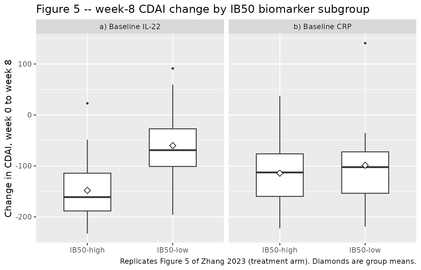

Assumptions and deviations

Baseline albumin units. Zhang 2023 Table 1 labels the albumin row “BALB, mg/dL” with median 39.0 and range 32.0-50.0. Those magnitudes are unambiguously g/L (normal serum albumin is roughly 35-50 g/L; 39 mg/dL would be a lethal hypoalbuminaemia), and the supplement analysis dataset column BALBU carries the same 32-50 range. The models use the canonical ALB in g/L with the published reference value 39 unchanged, so the published exponent -1.32 applies as printed. The “mg/dL” label is treated as a publication typo.
Sex coding. The source GNDR column is coded male = 1 / female = 0, whereas the canonical covariate is SEXF (1 = female). The published coefficient 0.214 is the male effect, so it is applied to (1 - SEXF). This preserves the paper’s female-reference typical value Vc = 3.27 L (males 3.97 L) rather than re-deriving a male-reference parameterisation.
Singular random-effect block. Table 2 reports the correlation between the baseline-CDAI and placebo-effect random effects as exactly -100%. A 2x2 covariance matrix with correlation -1 is singular (determinant 0) and rxode2’s Cholesky-based sampler fails on it with chol(): decomposition failed. The off-diagonal is therefore scaled by 0.99 (correlation -1.00 becomes -0.99); both published variances are kept exactly. This is the smallest perturbation that restores positive definiteness and it affects only the idealised “perfect correlation”, not any reported variance.
PK layer of the efficacy models. The supplement control streams PSP-2023-0072-T-s04.mod / s05.mod fix their PK thetas at values from an intermediate PK run (CL 0.239, Vc 3.23, …) carrying a different covariate structure (sex on CL, BMI on Vp) that the paper neither reports nor retained. Per the “final estimates, not initial estimates” rule, the two efficacy model files instead carry the final Table 2 PK parameters and the final covariate model, wrapped in fixed() to record that the PK was held constant while the efficacy parameters were estimated. This changes nothing about the CDAI predictions, because the drug effect is not exposure-driven (see next point).
The drug effect is not exposure-driven. Only one dose level (700 mg IV) was studied in phase IIa and the exposure range was narrow (5th-95th percentiles 43.7-106.1 ug/mL), so Zhang 2023 could not estimate a concentration-dependent drug effect and folded it into the biomarker-dependent term as a constant. The packaged models therefore gate the drug effect on ON_TREATMENT rather than on Cc. Consequently the PK layer does not feed the CDAI prediction; it is retained so a single model file simulates both endpoints.
cdai compartment name. The CDAI turnover state is declared via paper_specific_compartments rather than as a canonical compartment. It is the direct analogue of the registered das28 disease-activity-score output compartment and is a candidate for promotion to a canonical sibling in a future naming audit.
New canonical names. This extraction registers two new canonicals: the covariate IL22 (baseline serum interleukin-22, pg/mL, general scope; sibling of IL6 but a biologically distinct cytokine) and the parameter iplac (constant fractional placebo inhibition of an indirect-response production rate). Both were ratified by the operator before the model files were written.
Screened-but-unretained covariates. Baseline faecal calprotectin, IL-17, lipocalin-2, and MIP-3-alpha were screened as candidate biomarkers, and body weight, BMI, age, and race were screened in the PK stepwise covariate model; none were retained. They are documented in each model’s covariatesDataExcluded metadata so the provenance of the paper’s covariate screen is preserved without raising unused-covariate warnings.
Baseline CDAI is a parameter, not a covariate. The paper’s prognostic biomarker (BCDAI) enters the model as the estimated baseline parameter lrbase plus the -100% correlation between its random effect and the placebo effect’s – not as a covariate effect on any structural parameter. Figure 3 / Figure S2 report a post-hoc Pearson correlation between individual BCDAI and the individual estimated placebo effect, which is a diagnostic of that omega block. SCORE_CDAI is therefore recorded in covariatesDataExcluded.
Virtual cohort distributions. Baseline IL-22, CRP, and albumin distributions are log-normal / normal approximations calibrated to the published medians and clipped to the published observed ranges (Table 1); the paper does not report the full distributions. Sex is drawn as Bernoulli(0.622) for the phase IIa cohort and Bernoulli(0.118) for the phase Ib cohort. Race is not a model covariate and is not simulated.
Week-8 subgroup comparison. The simulated group means in the Figure 5 table will not match the published means exactly, because they depend on the simulated baseline-biomarker distribution rather than the 52 actual per-patient values. The quantity that is reproduced exactly is the plateau inhibition (the Figure 4 anchors table), which is a direct function of the published parameters.
No published NCA table. Zhang 2023 reports no Cmax / Tmax / AUC / half-life table, so the PKNCA section reports simulated values only, with the single published exposure metric (the 5th-95th percentile range of average concentration, 43.7-106.1 ug/mL) compared side by side. The paper does not state the averaging window for that range. It is quoted while discussing Figure S1, which plots each patient’s average concentration against their week-8 CDAI change, so the 0-56 day interval was taken as the matching window; it agrees to within 5% (45.5 and 111.0 ug/mL). The 0-84 day average is roughly 20-30% lower because no dose is given after day 29. Both are tabulated so the reader can see the effect of the window choice; no model parameter was adjusted.
Prediction-interval ribbons. The ribbons in the Figure 1a, 1b, and 1c replications are 5th-95th percentiles of individual model predictions (i.e. between-subject variability only), not full VPC intervals including residual error. The published Figure 1 panels show raw observed data and Figure S3 shows the VPCs; a like-for-like VPC would additionally sample the residual-error terms.
Errata. A search of the journal landing page and PubMed found no erratum, corrigendum, or author correction for doi:10.1002/psp4.13044 as of 2026-07-29.