Teduglutide (Marier 2010)

Model and source

• Citation: Marier JF, Mouksassi MS, Gosselin NH, Beliveau M, Cyran J, Wallens J. Population pharmacokinetics of teduglutide following repeated subcutaneous administrations in healthy participants and in patients with short bowel syndrome and Crohn’s disease. J Clin Pharmacol. 2010;50(1):36-49. doi:10.1177/0091270009342252
• Description: One-compartment population PK model with first-order subcutaneous absorption and a fixed absorption lag time for the GLP-2 analog teduglutide, fit to pooled data from eight phase I/II/III studies in healthy participants and in patients with short bowel syndrome, Crohn’s disease, or moderate hepatic impairment (Marier 2010). Site-specific typical absorption rate constant (abdomen vs pooled arm/thigh), a power effect of body weight on both apparent clearance and apparent central volume, and a categorical effect of sex on apparent clearance.
• Article: https://doi.org/10.1177/0091270009342252

Teduglutide (ALX-600, [gly2]-hGLP-2) is a synthetic analog of human glucagon-like peptide-2 carrying a single amino-acid substitution at the second N-terminal position, which confers resistance to degradation by dipeptidylpeptidase IV. Marier 2010 pooled eight phase I/II/III studies into a one-compartment population PK model with first-order subcutaneous absorption and a fixed absorption lag time. Two features distinguish it:

1. Site-specific absorption. Absorption from the abdomen is roughly 50% faster than from the arm or thigh, so the model carries two parallel typical absorption rate constants. Marier 2010 first fitted three injection-site categories and then pooled arm and thigh into one (Table III mod 16, dMOF = +1.552), so the packaged model uses two strata sharing one between-subject variability term.
2. A very steep body-weight effect on apparent volume. The power exponent of weight on Vc/F is 2.37 – far above any allometric expectation. The authors flag this themselves and it is the single largest driver of the reported half-life range.

The clinically load-bearing result is a negative one: neither renal function nor any marker of hepatic impairment explained variability in teduglutide PK, so no dose adjustment was deemed necessary in those populations. The screened and rejected covariates are recorded in the model file’s covariatesDataExcluded metadata so that provenance is not lost.

Population

The analysis pooled 266 participants from eight studies (Table I): five phase I studies in healthy adults (one of which, CL0600-017, enrolled 24 participants with moderate Child-Pugh class B hepatic impairment), two phase II studies (one in moderately active Crohn’s disease, one in short bowel syndrome), and one phase III study in parenteral-nutrition-dependent short bowel syndrome.

Baseline demographics come from Table II: mean age 39.1 years (median 38, range 18-79), mean weight 71.5 kg (median 70.9, range 40.1-127), and mean creatinine clearance 109 mL/min (range 26.0-236). There were 164 men (61.7%) and 102 women (38.3%). Participants were 83.8% white, 12.8% African American, 2.63% other, and 0.75% Asian. Of the 264 participants with a creatinine clearance, 60 (22.7%) fell in an impaired range (45 mild, 14 moderate, 1 severe).

Doses spanned 2.5 to 80 mg as fixed amounts and 0.03 to 0.20 mg/kg/day as weight-based amounts, given subcutaneously into the abdomen, arm or thigh, for durations from a single dose to 24 weeks. Plasma teduglutide was measured by LC/MS/MS over an analytical range of 1.00-120 ng/mL with an LOQ of 1.00 ng/mL.

pop <- rxode2::rxode(readModelDb("Marier_2010_teduglutide"))$population
#> ℹ parameter labels from comments will be replaced by 'label()'
str(pop, max.level = 1, give.attr = FALSE)
#> List of 18
#>  $ species         : chr "human"
#>  $ n_subjects      : int 266
#>  $ n_studies       : int 8
#>  $ age_range       : chr "18 - 79 years"
#>  $ age_median      : chr "38 years"
#>  $ age_mean        : chr "39.1 years"
#>  $ weight_range    : chr "40.1 - 127 kg"
#>  $ weight_median   : chr "70.9 kg"
#>  $ weight_mean     : chr "71.5 kg"
#>  $ sex_female_pct  : num 38.3
#>  $ race_ethnicity  : Named num [1:4] 83.8 12.8 2.63 0.75
#>  $ disease_state   : chr "Mixed: healthy participants (5 phase I studies), patients with moderately active Crohn's disease of at least 6 "| __truncated__
#>  $ dose_range      : chr "Daily subcutaneous teduglutide, 2.5 to 80 mg as fixed doses (2.5, 5, 7, 10, 15, 20, 25, 30, 50, 80 mg) and 0.03"| __truncated__
#>  $ renal_function  : chr "Creatinine clearance 26.0 - 236 mL/min (n = 264). 60 participants (22.7%) had creatinine clearance in an impair"| __truncated__
#>  $ hepatic_function: chr "Includes 24 participants with moderate (Child-Pugh class B, score 7-9) hepatic impairment from the dedicated st"| __truncated__
#>  $ regions         : chr "Not reported. Sponsor NPS Pharmaceuticals (Parsippany, NJ, USA); bioanalysis at Allelix Biopharmaceuticals (Mis"| __truncated__
#>  $ studies         : chr "ALX-0600 1621/1613 (phase I SAD, n = 32), CL0600-006 (phase I IV/SC bioavailability crossover, n = 14), CL0600-"| __truncated__
#>  $ notes           : chr "Demographics from Table II (n = 266; 164 men / 102 women). Estimation by NONMEM VI with FOCE-with-interaction. "| __truncated__

Source trace

Every ini() entry in inst/modeldb/specificDrugs/Marier_2010_teduglutide.R carries an in-file comment naming its source location. They are collected here for review.

Equation / parameter	Value	Source location
lka_abdomen	log(0.299) 1/h	Table V, Ka_abd (bootstrap 0.280-0.320); Table VI
lka_armthigh	log(0.206) 1/h	Table V, Ka_other (bootstrap 0.171-0.242); Table VI
lcl	log(12.4) L/h	Table V, CL/F (bootstrap 11.9-13.0); Table VI
lvc	log(32.8) L	Table V, Vc/F (bootstrap 30.6-34.9); Table VI
ltlag	fixed(log(0.208)) h	Table VI, ALAG = 0.208 (Fixed); Results, “Structural Model Buildup”
e_wt_vc	2.37	Table V, body weight on Vc/F (bootstrap 2.08-2.67); Table VI
e_wt_cl	0.323	Table V, body weight on CL/F (bootstrap 0.102-0.521); Table VI
e_sexf_cl	0.843	Table V, sex on CL/F (bootstrap 0.764-0.930); Table VI (12.4 -> 10.5 L/h)
reference weight 70.9 kg	n/a	Table VI denominator; equals the Table II median weight
etalka	log(0.395^2 + 1)	Table V, BSV on Ka = 39.5% (bootstrap 35.4-44.3)
etalcl	log(0.281^2 + 1)	Table V, BSV on CL/F = 28.1% (bootstrap 23.6-32.4)
etalvc	log(0.394^2 + 1)	Table V, BSV on Vc/F = 39.4% (bootstrap 32.5-45.7)
etaltlag	fixed(log(0.316^2 + 1))	Table VI, BSV on ALAG = 31.6% (fixed)
addSd	6.80 ng/mL	Table V, additive error (bootstrap 5.47-8.06)
propSd	0.243	Table V, proportional error = 24.3% (bootstrap 21.9-26.5)
1-compartment ODE, first-order absorption + lag	n/a	Results, “Structural Model Buildup”; Table III mod 2
Site-specific Ka, arm and thigh pooled	n/a	Table III mod 4 and mod 16
Power form for continuous covariates	n/a	Methods, “Covariate Analysis”
Combined additive + proportional residual error	n/a	Results, “Structural Model Buildup”

Packaged IIV round-trips to the published percentages

Marier 2010 heads its variability rows “BSV, %” and the Methods state that between-subject variability was an exponential random-effect model with lognormally distributed individual parameters, so the internal variance is omega^2 = log(CV^2 + 1). This is an exact identity, independent of any simulation, so it is asserted directly on the packaged omega matrix.

ui <- rxode2::rxode(readModelDb("Marier_2010_teduglutide"))
#> ℹ parameter labels from comments will be replaced by 'label()'
om <- ui$omega

published_bsv <- c(etalka = 39.5, etalcl = 28.1, etalvc = 39.4, etaltlag = 31.6)

bsv_chk <- tibble(
  eta       = names(published_bsv),
  published = as.numeric(published_bsv),
  omega2    = vapply(names(published_bsv), function(e) om[e, e], numeric(1)),
  recovered = 100 * sqrt(exp(omega2) - 1)
)
bsv_chk |>
  dplyr::rename(
    "Random effect"      = eta,
    "Published BSV (%)"  = published,
    "Packaged omega^2"   = omega2,
    "Recovered BSV (%)"  = recovered
  ) |>
  knitr::kable(digits = c(0, 1, 5, 2),
               caption = "Table V / Table VI BSV percentages recovered from the packaged omega matrix.")

Table V / Table VI BSV percentages recovered from the packaged omega matrix.

Random effect	Published BSV (%)	Packaged omega^2	Recovered BSV (%)
etalka	39.5	0.14499	39.5
etalcl	28.1	0.07600	28.1
etalvc	39.4	0.14430	39.4
etaltlag	31.6	0.09518	31.6

stopifnot(all(abs(bsv_chk$recovered - bsv_chk$published) < 0.01))

Structural checks that need no cohort

Three of the paper’s quantitative statements follow from the typical-value parameters alone. They are checked here before any simulation, because a transcription error in lka_*, lcl, lvc, e_wt_cl, e_wt_vc or e_sexf_cl breaks one of them immediately.

Absorption half-lives (Results, paragraph following Table V)

“Based on rate constants of absorption, half-lives of absorption of teduglutide in the abdomen and other areas (thigh and arm) were 2.32 and 3.36 hours, respectively.”

theta <- setNames(ui$theta, names(ui$theta))
ka_abd <- exp(theta[["lka_abdomen"]])
ka_oth <- exp(theta[["lka_armthigh"]])

abs_chk <- tibble(
  site      = c("Abdomen", "Arm or thigh"),
  ka        = c(ka_abd, ka_oth),
  t_half    = log(2) / c(ka_abd, ka_oth),
  published = c(2.32, 3.36)
)
abs_chk |>
  dplyr::rename("Injection site" = site, "Ka (1/h)" = ka,
                "Absorption t1/2 (h)" = t_half, "Published t1/2 (h)" = published) |>
  knitr::kable(digits = 3, caption = "Absorption half-lives (Marier 2010 Results).")

Absorption half-lives (Marier 2010 Results).

Injection site	Ka (1/h)	Absorption t1/2 (h)	Published t1/2 (h)
Abdomen	0.299	2.318	2.32
Arm or thigh	0.206	3.365	3.36

stopifnot(all(abs(abs_chk$t_half - abs_chk$published) < 0.005))

# "the rate constant of absorption was approximately 50% faster than that
# observed following administration in the arm and thigh"
pct_faster <- 100 * (ka_abd / ka_oth - 1)
stopifnot(pct_faster > 40, pct_faster < 60)
sprintf("Abdominal Ka is %.1f%% faster than arm/thigh (paper: 'approximately 50%%').", pct_faster)
#> [1] "Abdominal Ka is 45.1% faster than arm/thigh (paper: 'approximately 50%')."

Typical CL/F, Vc/F and elimination half-life by weight (Table VI narrative)

The paper states typical CL/F of 11.1 and 13.4 L/h and Vc/F of 14.3 and 57.7 L for 50 and 90 kg men, and elimination half-lives of 0.897 and 2.99 h. It also gives a typical female CL/F of 10.5 L/h at the reference weight.

wref <- 70.9

typ_cl <- function(wt, sexf) {
  exp(theta[["lcl"]]) * (wt / wref)^theta[["e_wt_cl"]] * theta[["e_sexf_cl"]]^sexf
}
typ_vc <- function(wt) exp(theta[["lvc"]]) * (wt / wref)^theta[["e_wt_vc"]]

t6 <- tibble(
  wt          = c(50, 90),
  cl          = typ_cl(wt, 0),
  cl_pub      = c(11.1, 13.4),
  vc          = typ_vc(wt),
  vc_pub      = c(14.3, 57.7),
  t_half      = log(2) * vc / cl,
  t_half_pub  = c(0.897, 2.99)
)
t6 |>
  dplyr::rename("Weight (kg)" = wt, "CL/F (L/h)" = cl, "Published CL/F" = cl_pub,
                "Vc/F (L)" = vc, "Published Vc/F" = vc_pub,
                "t1/2 (h)" = t_half, "Published t1/2" = t_half_pub) |>
  knitr::kable(digits = 3, caption = "Table VI narrative values for men, reproduced from the packaged thetas.")

Table VI narrative values for men, reproduced from the packaged thetas.

Weight (kg)	CL/F (L/h)	Published CL/F	Vc/F (L)	Published Vc/F	t1/2 (h)	Published t1/2
50	11.077	11.1	14.335	14.3	0.897	0.897
90	13.393	13.4	57.729	57.7	2.988	2.990

# Published to 3 significant figures, so match to within half a printed unit
# in the last place of each quantity.
stopifnot(
  all(abs(t6$cl     - t6$cl_pub)     < 0.05),
  all(abs(t6$vc     - t6$vc_pub)     < 0.05),
  all(abs(t6$t_half - t6$t_half_pub) < 0.005)
)

cl_female_ref <- typ_cl(wref, 1)
stopifnot(abs(cl_female_ref - 10.5) < 0.05)
sprintf("Typical female CL/F at %.1f kg = %.3f L/h (paper: 10.5 L/h, i.e. 12.4 x 0.843).",
        wref, cl_female_ref)
#> [1] "Typical female CL/F at 70.9 kg = 10.453 L/h (paper: 10.5 L/h, i.e. 12.4 x 0.843)."

Virtual cohort

Original observed data are not publicly available. Two cohorts are built.

Cohort T (typical-value grid). Table VII of Marier 2010 tabulates predicted steady-state AUC and Cmax for six sex-by-weight combinations, two dose levels (0.05 and 0.10 mg/kg/day), and two injection sites. This is a typical-value prediction, so it is reproduced with the random effects zeroed: one subject per published cell, 24 cells in total. This is the vignette’s primary quantitative gate.

Cohort V (stochastic). A 200-subject-per-arm cohort with sampled weight and sex, used for the concentration-time figure and for the minimal-accumulation check. 200 per arm is the skill’s cap and is ample here.

tau     <- 24    # daily subcutaneous dosing
n_doses <- 10L   # ample for a drug whose longest typical t1/2 is ~5.4 h
t_last  <- tau * (n_doses - 1L)

# Table VII, transcribed verbatim. Cmax is site-specific; AUC is not, because
# total exposure does not depend on the absorption rate constant.
table7 <- tibble::tribble(
  ~sex,     ~wt, ~mgkg, ~auc, ~cmax_abdomen, ~cmax_armthigh,
  "Men",     40, 0.05,  194,  36.8,          28.1,
  "Men",     70, 0.05,  283,  35.4,          29.0,
  "Men",    120, 0.05,  408,  30.1,          26.9,
  "Women",   40, 0.05,  229,  41.4,          31.9,
  "Women",   60, 0.05,  302,  40.2,          32.6,
  "Women",   90, 0.05,  397,  35.7,          30.8,
  "Men",     40, 0.10,  388,  73.6,          56.2,
  "Men",     70, 0.10,  567,  70.8,          57.9,
  "Men",    120, 0.10,  816,  60.3,          53.7,
  "Women",   40, 0.10,  458,  82.8,          63.8,
  "Women",   60, 0.10,  603,  80.5,          65.1,
  "Women",   90, 0.10,  794,  71.5,          61.5
)

# One arm per (sex, weight, dose level, injection site).
grid_t <- table7 |>
  dplyr::select(sex, wt, mgkg) |>
  tidyr::crossing(site = c("abdomen", "armthigh")) |>
  dplyr::mutate(
    id       = dplyr::row_number(),
    SEXF     = as.integer(sex == "Women"),
    WT       = wt,
    # INJSITE_ARM and INJSITE_THIGH are pooled by the model into a single
    # non-abdomen stratum; the arm/thigh arms are represented by the thigh
    # indicator, which carries most of the patient data in the source studies.
    INJSITE_ARM   = 0L,
    INJSITE_THIGH = as.integer(site == "armthigh"),
    amt_mg   = mgkg * wt,
    treatment = sprintf("%s %d kg, %.2f mg/kg, %s", sex, wt, mgkg, site)
  )

# Dose records: n_doses daily doses into `depot`.
dose_t <- grid_t |>
  tidyr::crossing(time = seq(0, t_last, by = tau)) |>
  dplyr::mutate(evid = 1L, cmt = "depot", amt = amt_mg)

# Observation records over the final (steady-state) dosing interval. The grid is
# dense where the peak sits and coarser thereafter: a coarse grid makes max(Cc)
# a discretisation artefact even while the integrator states stay exact.
obs_times <- sort(unique(c(
  t_last + seq(0,  8, by = 0.02),
  t_last + seq(8, tau, by = 0.25)
)))
obs_t <- grid_t |>
  tidyr::crossing(time = obs_times) |>
  # `cmt` on an observation row must be an ODE STATE, never the algebraic
  # observable `Cc`; rxode2 returns Cc as a column regardless.
  dplyr::mutate(evid = 0L, cmt = "central", amt = NA_real_)

events_t <- dplyr::bind_rows(dose_t, obs_t) |>
  dplyr::arrange(id, time, dplyr::desc(evid)) |>
  dplyr::select(id, time, amt, evid, cmt, WT, SEXF, INJSITE_ARM, INJSITE_THIGH, treatment)

stopifnot(
  !anyDuplicated(unique(events_t[, c("id", "time", "evid")])),
  nrow(dplyr::distinct(grid_t, id)) == 24L
)

rxode2::rxSetSeed(20260826)
set.seed(20260826)

n_arm <- 200L

# Weight sampled to match Table II: median 70.9 kg, mean 71.5 kg, SD 15.8 kg,
# range 40.1-127 kg. A lognormal reproduces the slight right skew implied by
# mean > median and is truncated to the observed range.
sample_wt <- function(n) {
  sdlog   <- sqrt(log1p((15.8 / 71.5)^2))
  meanlog <- log(70.9)
  wt <- rlnorm(n, meanlog, sdlog)
  pmin(pmax(wt, 40.1), 127)
}

make_arm <- function(n, mgkg, site, label, id_offset) {
  subj <- tibble(
    id            = id_offset + seq_len(n),
    WT            = sample_wt(n),
    SEXF          = rbinom(n, 1L, 0.383),   # Table II: 38.3% women
    INJSITE_ARM   = 0L,
    INJSITE_THIGH = as.integer(site == "armthigh"),
    treatment     = label
  ) |>
    dplyr::mutate(amt_mg = mgkg * WT)

  dplyr::bind_rows(
    subj |> tidyr::crossing(time = seq(0, t_last, by = tau)) |>
      dplyr::mutate(evid = 1L, cmt = "depot", amt = amt_mg),
    subj |> tidyr::crossing(time = sort(unique(c(
      seq(0, tau, by = 0.25),                 # first interval, for Figure 1A
      t_last + seq(0, tau, by = 0.25)         # steady state, for Figure 1B
    )))) |>
      dplyr::mutate(evid = 0L, cmt = "central", amt = NA_real_)
  ) |>
    dplyr::arrange(id, time, dplyr::desc(evid))
}

events_v <- dplyr::bind_rows(
  make_arm(n_arm, 0.05, "abdomen", "0.05 mg/kg, abdomen", id_offset =      0L),
  make_arm(n_arm, 0.10, "abdomen", "0.10 mg/kg, abdomen", id_offset =  n_arm),
  make_arm(n_arm, 0.10, "armthigh", "0.10 mg/kg, arm/thigh", id_offset = 2L * n_arm)
) |>
  dplyr::select(id, time, amt, evid, cmt, WT, SEXF, INJSITE_ARM, INJSITE_THIGH, treatment)

stopifnot(!anyDuplicated(unique(events_v[, c("id", "time", "evid")])))

Simulation

mod <- readModelDb("Marier_2010_teduglutide")

# Cohort T: typical-value replication of Table VII, random effects zeroed.
mod_typ <- mod |> rxode2::zeroRe()
#> ℹ parameter labels from comments will be replaced by 'label()'
sim_t <- rxode2::rxSolve(
  mod_typ, events = events_t,
  keep = c("WT", "SEXF", "INJSITE_THIGH", "treatment")
) |>
  as.data.frame()
#> ℹ omega/sigma items treated as zero: 'etalka', 'etalcl', 'etalvc', 'etaltlag'
#> Warning: multi-subject simulation without without 'omega'

# Confirm zeroRe() also zeroed the FIXED lag-time eta, so tlag is the
# published 0.208 h rather than a sampled value.
stopifnot(all(abs(sim_t$tlag - 0.208) < 1e-8))

# Cohort V: stochastic, for the figures and the accumulation check.
sim_v <- rxode2::rxSolve(
  mod, events = events_v,
  keep = c("WT", "SEXF", "treatment")
) |>
  as.data.frame()
#> ℹ parameter labels from comments will be replaced by 'label()'

stopifnot(nrow(sim_t) > 0, nrow(sim_v) > 0, all(sim_t$Cc >= 0))

The individual cl and vc values that rxode2 computed in the typical-value solve are the same closed-form quantities checked above; confirming them inside the solve closes the loop between the packaged thetas and the ODE system.

par_chk <- sim_t |>
  dplyr::distinct(id, WT, SEXF, cl, vc) |>
  dplyr::mutate(
    cl_expected = typ_cl(WT, SEXF),
    vc_expected = typ_vc(WT)
  )
stopifnot(
  all(abs(par_chk$cl - par_chk$cl_expected) < 1e-8),
  all(abs(par_chk$vc - par_chk$vc_expected) < 1e-8)
)
sprintf("cl and vc in the solve match the closed form for all %d typical-value arms.",
        nrow(par_chk))
#> [1] "cl and vc in the solve match the closed form for all 24 typical-value arms."

Replicate published figures

Figure 1 – plasma concentrations after single and repeated SC dosing

Figure 1 of Marier 2010 is a scatterplot of individual plasma concentrations after (A) single and (B) repeated subcutaneous administration, overlaid with a LOESS curve. The published narrative is that concentrations decline mono-exponentially and that most fall below the 1.00 ng/mL assay limit by 24 h postdose. The panels below are the simulated equivalent: median with a 5th-95th percentile ribbon, on a log scale, with the assay LOQ marked.

fig1 <- sim_v |>
  dplyr::mutate(
    panel = ifelse(time <= tau, "(A) First dose", "(B) Steady state (dose 10)"),
    tad   = ifelse(time <= tau, time, time - t_last)
  ) |>
  dplyr::group_by(panel, treatment, tad) |>
  dplyr::summarise(
    Q05 = quantile(Cc, 0.05),
    Q50 = quantile(Cc, 0.50),
    Q95 = quantile(Cc, 0.95),
    .groups = "drop"
  )

ggplot(fig1, aes(tad, Q50, colour = treatment, fill = treatment)) +
  geom_ribbon(aes(ymin = pmax(Q05, 0.05), ymax = Q95), alpha = 0.18, colour = NA) +
  geom_line(linewidth = 0.7) +
  geom_hline(yintercept = 1.0, linetype = "dashed", colour = "grey40") +
  facet_wrap(~panel) +
  scale_y_log10() +
  labs(
    x = "Time after dose (h)", y = "Teduglutide Cc (ng/mL)",
    colour = NULL, fill = NULL,
    title = "Figure 1 -- simulated plasma teduglutide, single and repeated SC dosing",
    caption = paste("Replicates Figure 1 of Marier 2010. Dashed line is the 1.00 ng/mL assay LOQ.",
                    "Median with 5th-95th percentile ribbon,", n_arm, "subjects per arm.")
  ) +
  theme_bw() +
  theme(legend.position = "bottom")
#> Warning in scale_y_log10(): log-10 transformation introduced infinite values.
#> log-10 transformation introduced infinite values.
#> log-10 transformation introduced infinite values.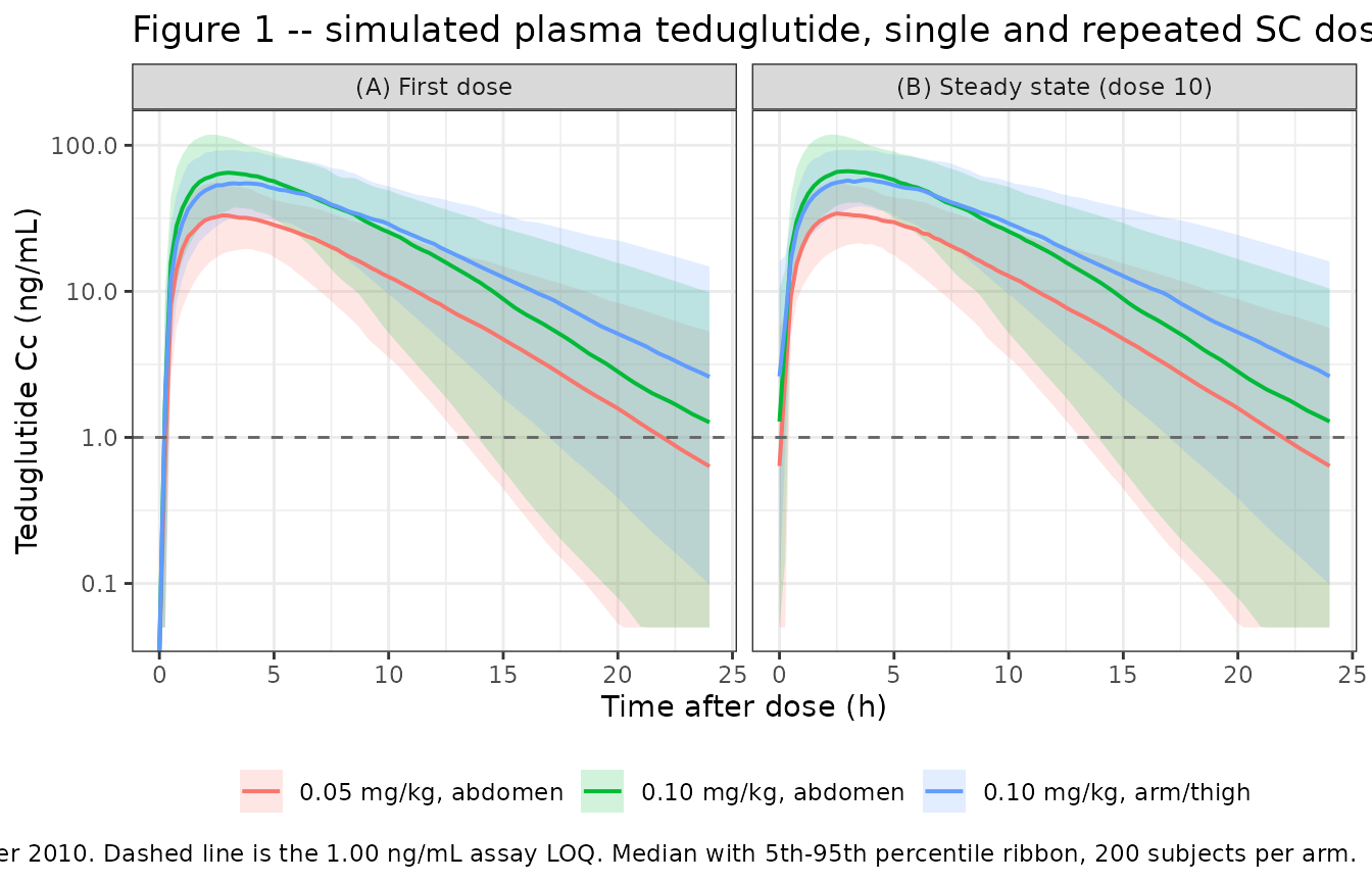

Minimal accumulation on daily dosing

Marier 2010 reports that “approximately 60 blood samples of 183 (32.8%) displayed measurable predose concentration values of teduglutide following repeated administrations”, and concludes that “multiple SC administrations of teduglutide resulted in a very minor accumulation of the drug”.

This is a genuine check on the joint magnitude of the elimination rate, the between-subject variability and the residual error, but it is only approximate: the published 32.8% comes from the actual pooled sampling schedule and dose mix, which cannot be reconstructed. It is reported here with a deliberately wide band and is not treated as a tight gate.

# Steady-state trough (predose for the notional 11th dose) vs the LOQ, on
# residual-error-carrying observations.
trough <- sim_v |>
  dplyr::filter(abs(time - (t_last + tau)) < 1e-8) |>
  dplyr::mutate(
    Cc_obs = Cc * (1 + rnorm(dplyr::n(), 0, 0.243)) + rnorm(dplyr::n(), 0, 6.80)
  )

acc <- sim_v |>
  dplyr::group_by(id) |>
  dplyr::summarise(
    peak_first = max(Cc[time <= tau]),
    peak_ss    = max(Cc[time >= t_last]),
    .groups    = "drop"
  ) |>
  dplyr::mutate(ratio = peak_ss / peak_first)

pct_measurable <- 100 * mean(trough$Cc_obs > 1.0)

tibble(
  Quantity = c("Measurable steady-state troughs (> 1.00 ng/mL)",
               "Median peak accumulation ratio (dose 10 / dose 1)",
               "90th percentile peak accumulation ratio"),
  Simulated = c(sprintf("%.1f%%", pct_measurable),
                sprintf("%.3f", median(acc$ratio)),
                sprintf("%.3f", quantile(acc$ratio, 0.9))),
  Published = c("32.8% (60 of 183 samples)", "'very minor accumulation'", "--")
) |>
  knitr::kable(caption = "Accumulation on daily SC dosing (Marier 2010 Results, 'Structural Model Buildup').")

Accumulation on daily SC dosing (Marier 2010 Results, ‘Structural Model Buildup’).

Quantity	Simulated	Published
Measurable steady-state troughs (> 1.00 ng/mL)	55.8%	32.8% (60 of 183 samples)
Median peak accumulation ratio (dose 10 / dose 1)	1.012	‘very minor accumulation’
90th percentile peak accumulation ratio	1.085	–

stopifnot(
  # Accumulation is minimal: the median subject gains at most a few percent.
  median(acc$ratio) > 1.0,
  median(acc$ratio) < 1.10,
  quantile(acc$ratio, 0.9) < 1.35,
  # Wide band; see the caveat above.
  pct_measurable > 5, pct_measurable < 65
)

PKNCA validation

Steady-state NCA over the final dosing interval of the typical-value grid (recipe 3 of pknca-recipes.md). The grouping variable is the sex-by-weight-by-dose-by-site arm, which is exactly the stratification of Table VII.

sim_nca <- sim_t |>
  dplyr::filter(!is.na(Cc)) |>
  dplyr::select(id, time, Cc, treatment)

# No defensive time-zero row is needed here, because the interval starts at
# t_last and that is itself a real observation (the steady-state trough), so
# PKNCA has an anchor for AUC0-tau. Confirm every arm actually has that row --
# otherwise PKNCA emits the "AUC range starting before the first measurement"
# warning once per subject.
anchor_arms <- sim_nca |>
  dplyr::filter(abs(time - t_last) < 1e-8) |>
  dplyr::distinct(treatment)
stopifnot(nrow(anchor_arms) == 24L)

conc_obj <- PKNCA::PKNCAconc(
  sim_nca, Cc ~ time | treatment + id,
  concu = "ng/mL", timeu = "h"
)

dose_df <- events_t |>
  dplyr::filter(evid == 1) |>
  dplyr::select(id, time, amt, treatment)

dose_obj <- PKNCA::PKNCAdose(dose_df, amt ~ time | treatment + id, doseu = "mg")

intervals <- data.frame(
  start   = t_last,
  end     = t_last + tau,
  cmax    = TRUE,
  tmax    = TRUE,
  cmin    = TRUE,
  auclast = TRUE,
  cav     = TRUE
)

nca_res <- PKNCA::pk.nca(PKNCA::PKNCAdata(conc_obj, dose_obj, intervals = intervals))

Comparison against published NCA (Table VII)

Table VII is a typical-value prediction, so the comparison is against the zeroed-random-effect solve and the difference is pure numerical error plus the paper’s own printed rounding – not cohort sampling noise. A tight bound is therefore the correct gate here, and it is asserted over all 36 published cells of Table VII: the 24 Cmax values, plus the 12 AUC values (which Table VII reports once per sex/weight/dose because total exposure does not depend on the absorption rate constant, so each is checked against both injection-site arms).

The paper prints three significant figures and its inputs are themselves three-figure values; the dominant propagated term is the rounding of the sex coefficient 0.843, worth about 0.06%. A 2% bound leaves ample headroom while still catching any real transcription error, which would move a value by tens of percent.

published <- table7 |>
  tidyr::pivot_longer(c(cmax_abdomen, cmax_armthigh),
                      names_to = "site", values_to = "cmax") |>
  dplyr::mutate(
    site      = sub("^cmax_", "", site),
    treatment = sprintf("%s %d kg, %.2f mg/kg, %s", sex, wt, mgkg, site),
    auclast   = auc
  ) |>
  dplyr::select(treatment, cmax, auclast)

cmp <- nlmixr2lib::ncaComparisonTable(
  simulated     = nca_res,
  reference     = published,
  by            = "treatment",
  params        = c("cmax", "auclast"),
  units         = c(cmax = "ng/mL", auclast = "ng*h/mL"),
  tolerance_pct = 2
)

knitr::kable(
  cmp,
  caption = paste("Simulated steady-state NCA vs Marier 2010 Table VII.",
                  "* flags a >2% difference from the published value."),
  digits  = 3
)

Simulated steady-state NCA vs Marier 2010 Table VII. * flags a >2% difference from the published value.

NCA parameter	treatment	Reference	Simulated	% diff
Cmax (ng/mL)	Men 40 kg, 0.05 mg/kg, abdomen	36.8	36.8	-0.0%
Cmax (ng/mL)	Men 40 kg, 0.05 mg/kg, armthigh	28.1	28.1	-0.0%
Cmax (ng/mL)	Men 70 kg, 0.05 mg/kg, abdomen	35.4	35.4	+0.1%
Cmax (ng/mL)	Men 70 kg, 0.05 mg/kg, armthigh	29	29	-0.2%
Cmax (ng/mL)	Men 120 kg, 0.05 mg/kg, abdomen	30.1	30.1	+0.1%
Cmax (ng/mL)	Men 120 kg, 0.05 mg/kg, armthigh	26.9	26.9	-0.1%
Cmax (ng/mL)	Women 40 kg, 0.05 mg/kg, abdomen	41.4	41.5	+0.3%
Cmax (ng/mL)	Women 40 kg, 0.05 mg/kg, armthigh	31.9	32	+0.3%
Cmax (ng/mL)	Women 60 kg, 0.05 mg/kg, abdomen	40.2	40.3	+0.4%
Cmax (ng/mL)	Women 60 kg, 0.05 mg/kg, armthigh	32.6	32.6	+0.1%
Cmax (ng/mL)	Women 90 kg, 0.05 mg/kg, abdomen	35.7	35.8	+0.3%
Cmax (ng/mL)	Women 90 kg, 0.05 mg/kg, armthigh	30.8	30.9	+0.2%
Cmax (ng/mL)	Men 40 kg, 0.10 mg/kg, abdomen	73.6	73.6	-0.0%
Cmax (ng/mL)	Men 40 kg, 0.10 mg/kg, armthigh	56.2	56.2	-0.0%
Cmax (ng/mL)	Men 70 kg, 0.10 mg/kg, abdomen	70.8	70.8	+0.1%
Cmax (ng/mL)	Men 70 kg, 0.10 mg/kg, armthigh	57.9	57.9	+0.0%
Cmax (ng/mL)	Men 120 kg, 0.10 mg/kg, abdomen	60.3	60.3	-0.0%
Cmax (ng/mL)	Men 120 kg, 0.10 mg/kg, armthigh	53.7	53.7	+0.1%
Cmax (ng/mL)	Women 40 kg, 0.10 mg/kg, abdomen	82.8	83.1	+0.3%
Cmax (ng/mL)	Women 40 kg, 0.10 mg/kg, armthigh	63.8	64	+0.3%
Cmax (ng/mL)	Women 60 kg, 0.10 mg/kg, abdomen	80.5	80.7	+0.2%
Cmax (ng/mL)	Women 60 kg, 0.10 mg/kg, armthigh	65.1	65.3	+0.3%
Cmax (ng/mL)	Women 90 kg, 0.10 mg/kg, abdomen	71.5	71.6	+0.2%
Cmax (ng/mL)	Women 90 kg, 0.10 mg/kg, armthigh	61.5	61.7	+0.3%
AUClast (ng*h/mL)	Men 40 kg, 0.05 mg/kg, abdomen	194	194	+0.0%
AUClast (ng*h/mL)	Men 40 kg, 0.05 mg/kg, armthigh	194	194	+0.0%
AUClast (ng*h/mL)	Men 70 kg, 0.05 mg/kg, abdomen	283	283	+0.1%
AUClast (ng*h/mL)	Men 70 kg, 0.05 mg/kg, armthigh	283	283	+0.1%
AUClast (ng*h/mL)	Men 120 kg, 0.05 mg/kg, abdomen	408	408	+0.1%
AUClast (ng*h/mL)	Men 120 kg, 0.05 mg/kg, armthigh	408	408	+0.1%
AUClast (ng*h/mL)	Women 40 kg, 0.05 mg/kg, abdomen	229	230	+0.5%
AUClast (ng*h/mL)	Women 40 kg, 0.05 mg/kg, armthigh	229	230	+0.5%
AUClast (ng*h/mL)	Women 60 kg, 0.05 mg/kg, abdomen	302	303	+0.3%
AUClast (ng*h/mL)	Women 60 kg, 0.05 mg/kg, armthigh	302	303	+0.3%
AUClast (ng*h/mL)	Women 90 kg, 0.05 mg/kg, abdomen	397	399	+0.4%
AUClast (ng*h/mL)	Women 90 kg, 0.05 mg/kg, armthigh	397	399	+0.4%
AUClast (ng*h/mL)	Men 40 kg, 0.10 mg/kg, abdomen	388	388	+0.0%
AUClast (ng*h/mL)	Men 40 kg, 0.10 mg/kg, armthigh	388	388	+0.0%
AUClast (ng*h/mL)	Men 70 kg, 0.10 mg/kg, abdomen	567	567	-0.0%
AUClast (ng*h/mL)	Men 70 kg, 0.10 mg/kg, armthigh	567	567	-0.0%
AUClast (ng*h/mL)	Men 120 kg, 0.10 mg/kg, abdomen	816	816	+0.1%
AUClast (ng*h/mL)	Men 120 kg, 0.10 mg/kg, armthigh	816	816	+0.1%
AUClast (ng*h/mL)	Women 40 kg, 0.10 mg/kg, abdomen	458	460	+0.5%
AUClast (ng*h/mL)	Women 40 kg, 0.10 mg/kg, armthigh	458	460	+0.5%
AUClast (ng*h/mL)	Women 60 kg, 0.10 mg/kg, abdomen	603	606	+0.5%
AUClast (ng*h/mL)	Women 60 kg, 0.10 mg/kg, armthigh	603	606	+0.5%
AUClast (ng*h/mL)	Women 90 kg, 0.10 mg/kg, abdomen	794	797	+0.4%
AUClast (ng*h/mL)	Women 90 kg, 0.10 mg/kg, armthigh	794	797	+0.4%

# Recompute the percent differences directly so the gate does not depend on the
# comparison table's presentation columns.
sim_wide <- as.data.frame(nca_res) |>
  dplyr::filter(PPTESTCD %in% c("cmax", "auclast")) |>
  dplyr::select(treatment, PPTESTCD, PPORRES) |>
  tidyr::pivot_wider(names_from = PPTESTCD, values_from = PPORRES)

gate <- published |>
  dplyr::rename(cmax_pub = cmax, auclast_pub = auclast) |>
  dplyr::inner_join(sim_wide, by = "treatment") |>
  dplyr::mutate(
    cmax_pct = 100 * (cmax    - cmax_pub)    / cmax_pub,
    auc_pct  = 100 * (auclast - auclast_pub) / auclast_pub
  )

# Guard against a silently empty join: a lookup that matches no rows would make
# every all() below vacuously TRUE.
stopifnot(nrow(gate) == 24L, !anyNA(gate$cmax_pct), !anyNA(gate$auc_pct))

# 24 arms x 2 parameters = 48 comparisons, covering all 36 distinct published
# numbers: 24 Cmax cells, plus the 12 AUC cells each checked at both injection
# sites (Table VII prints one AUC per sex/weight/dose because AUC does not
# depend on the absorption rate constant).
sprintf(paste("Table VII reproduction: %d comparisons over %d arms, covering all 36 published",
              "cells. Max |%%diff| = %.2f%% (Cmax), %.2f%% (AUC0-tau) -- %.0f%% of the 2%% budget."),
        2L * nrow(gate), nrow(gate), max(abs(gate$cmax_pct)), max(abs(gate$auc_pct)),
        100 * max(abs(c(gate$cmax_pct, gate$auc_pct))) / 2)
#> [1] "Table VII reproduction: 48 comparisons over 24 arms, covering all 36 published cells. Max |%diff| = 0.35% (Cmax), 0.52% (AUC0-tau) -- 26% of the 2% budget."

stopifnot(
  all(abs(gate$cmax_pct) < 2),
  all(abs(gate$auc_pct)  < 2)
)

The AUC arm of that gate is also a closed-form mass-balance check: at steady state AUC0-tau equals Dose / (CL/F) exactly, so agreement with Table VII confirms both the clearance model and the trapezoidal integration.

mb <- sim_t |>
  dplyr::distinct(id, treatment, WT, SEXF, cl) |>
  dplyr::left_join(
    dose_df |> dplyr::distinct(id, amt),
    by = "id"
  ) |>
  dplyr::left_join(
    sim_wide |> dplyr::select(treatment, auclast),
    by = "treatment"
  ) |>
  dplyr::mutate(
    auc_closed = amt / cl * 1000,               # mg / (L/h) -> ng*h/mL
    pct        = 100 * (auclast - auc_closed) / auc_closed
  )

stopifnot(nrow(mb) == 24L, all(abs(mb$pct) < 0.5))
sprintf("AUC0-tau,ss vs Dose/(CL/F): max |%%diff| = %.3f%% across %d arms.",
        max(abs(mb$pct)), nrow(mb))
#> [1] "AUC0-tau,ss vs Dose/(CL/F): max |%diff| = 0.002% across 24 arms."

Assumptions and deviations

• Ka encoded as two parallel strata, not a reference plus an offset. Table V reports Ka_abd and Ka_other as two typical values each with its own bootstrap percentile interval, listed under “Population PK Parameters” rather than under “Covariate model”, so they are encoded as the stratum-suffixed lka_abdomen / lka_armthigh pair. The single Table V BSV on Ka of 39.5% is shared between the strata, matching the paper’s one reported value.

• Arm and thigh pooled via the sum of two canonical indicators. The registered INJSITE_<site> family has mutually exclusive members with all-zero denoting the abdomen reference, so injsite_nonabd = INJSITE_ARM + INJSITE_THIGH is already the 0/1 non-abdomen indicator that Marier 2010’s pooled stratum needs. No INJSITE_OTHER canonical was introduced; keeping both source columns preserves which anatomical sites the cohort actually used. In the typical-value grid the arm/thigh arms are represented by INJSITE_THIGH = 1.

• Reference weight 70.9 kg is the cohort median, not the mean. Table II gives a mean of 71.5 kg and a median of 70.9 kg; Table VI writes the denominator as 70.9. Reproducing the Table VI half-lives and all 36 Table VII cells confirms the median is the normalising value.

• BSV, % read as a coefficient of variation on the lognormal, giving omega^2 = log(CV^2 + 1). The paper does not name the convention. Two candidate readings were considered and one was ruled out:

  • Ruled out: the percentages are raw omega^2 values scaled by 100. Adding a covariate that reduces a random effect’s unexplained variance from omega^2_0 to omega^2_1 can reduce the objective function by at most about N * log(omega^2_0 / omega^2_1) for N = 266 subjects, and less once shrinkage is accounted for. On the variance reading, Table IV mod7 (weight on Vc/F, BSV 59 -> 39) admits at most 110 units but the paper reports dMOF = -167.854, and mod13 (sex on CL/F, BSV 32 -> 29) admits at most 26 against a reported -30.318. Both observed drops exceed the ceiling, so the numbers cannot be variances. On the CV reading the same two steps admit 199 and 50 units respectively, comfortably above what was observed.
  • Retained: exact lognormal CV, omega^2 = log(CV^2 + 1). This is the nlmixr2lib convention. The alternative approximation omega = CV / 100 is not discriminated by anything the paper prints, but it differs by less than 4% in omega at the largest reported BSV (0.395 vs 0.381 for Ka), so the choice is immaterial for simulation.

• Residual error read on the SD scale. Table V prints the two error terms in SD-scale units, “Additive error, ng/mL” and “Proportional error, %”, so they are used directly as addSd = 6.80 and propSd = 0.243 with no sqrt(). Corroboration from the bootstrap-CI relative width: with subject-level resampling of n = 266, an SD-scale estimate predicts a relative 95% interval width near 3.92 * sqrt(1 / (2 * 266)) = 0.170 and a variance-scale estimate twice that. The proportional row’s observed width is (26.5 - 21.9) / 24.2 = 0.190, matching the SD prediction and 1.8x away from the variance prediction. The additive row is wider (0.385), which is expected because only the minority of samples near the 1.00 ng/mL LOQ inform an additive term, so its effective sample size is well below 266.

• ALAG and its BSV are both fixed(). Results, “Structural Model Buildup”: “The absorption lag time (ALAG) as well as BSV were fixed to population values previously estimated with the model to stabilize the model and facilitate convergence”, and Table VI prints “0.208 (Fixed)” and “31.6 (fixed)”. Consistently, neither appears in the Table V bootstrap. The “population values previously estimated with the model” are not tabulated anywhere in the paper as a separate provenance, so the Table VI numbers are taken as the values themselves.

• No bioavailability parameter. The model is parameterised in apparent terms (CL/F, Vc/F), so F is absorbed into those. Marier 2010 tested site of administration on relative bioavailability (Table III mod 6) and did not retain it. The paper separately notes that an assumed SC bioavailability of 87% would put the true volume near 28.5 L, but that scaling is commentary and is not part of the fitted model.

• Table VII Cmax is a steady-state quantity. The table is headed only “Predicted AUC and Cmax Values of Teduglutide According to Patient Demographics”, but its Cmax values are reproduced by the steady-state expression over a 24 h interval and not by the single-dose one. The difference is small because accumulation is minimal, but it is resolvable: for the 120 kg men at 0.05 mg/kg the single-dose value is 27.8 ng/mL against a published 30.1, while the steady-state value is 30.2. All arms are therefore simulated to steady state (dose 10 of 10).

• Covariate distributions assumed. Weight is drawn from a lognormal matched to the Table II mean (71.5 kg), median (70.9 kg) and SD (15.8 kg), truncated to the observed 40.1-127 kg range; the paper reports no distributional form. Sex is Bernoulli at the Table II 38.3% female. Neither assumption affects the Table VII gate, which uses the paper’s own weights directly.

• Only two of the eight studies’ injection sites are represented in the stochastic cohort. Site was recorded per administration in the source data; the simulated arms hold it constant per subject, which is adequate for the figures but does not reproduce the CL0600-015 three-way crossover design.

Errata

• The Abstract’s participant count disagrees with the Results. The Abstract states that PK “were assessed following daily subcutaneous (SC) administrations of 2.5 to 80 mg doses in a total of 256 patients”, but the Results section states that “Plasma concentration-time profiles of teduglutide from a total of 266 participants were available to build the structural model”, Table II reports n = 266 for age and weight, and the demographic narrative gives “164 men (61.7%) and 102 women (38.3%)”, which sums to 266. The model file records n_subjects = 266L; the Abstract’s 256 appears to be a typographical error.

• The Abstract’s direction of the sex effect reads oddly against its own numbers. The Abstract says clearance “in male participants was approximately 18% higher than that observed in female participants (12.4 vs 10.5 L/h, respectively)”, which is consistent with 12.4 / 10.5 = 1.18. The Results then say the effect “was not deemed clinically relevant because male participants are expected to display teduglutide exposure values (AUC) approximately 18% lower than female participants” – the same 18%, correctly inverted for exposure. Both statements are consistent with e_sexf_cl = 0.843; no correction is needed, but the two “18%” figures describe different quantities.

• Table III is garbled in the machine-readable rendering of the PDF. Rows mod 3 and mod 7 through mod 15 are absent and two rows are replaced by repeated copies of a section header. The rows that survive (mod 1, mod 2, mod 4, mod 5, mod 6, mod 16, mod 17) are sufficient to establish the structural-model narrative used here – first-order absorption with a lag time beats without (dMOF = -598.313), site of administration acts on Ka rather than on ALAG or Frel (-100.824 vs -47.896 and -50.780), and collapsing three injection-site categories to two costs only +1.552. No parameter value in the model file depends on a missing row.

• No erratum or corrigendum was located. A search of the article’s landing page at the publisher and of the DOI record surfaced no correction notice for doi:10.1177/0091270009342252.