Model and source
- Citation: Kim YK, Kim D, Kang G, Zang DY, Lee DH.Pharmacokinetics of Vancomycin in Healthy Korean Volunteers and Monte Carlo Simulations to Explore Optimal Dosage Regimens in Patients with Normal Renal Function. Antibiotics (Basel). 2024;13(10):993. doi:10.3390/antibiotics13100993
- Description: Two-compartment IV population PK model for vancomycin in healthy Korean adult volunteers (Kim 2024). Clearance scales as power functions of body weight (exponent 1.28, reference 69.45 kg) and age (exponent -0.377, reference 38.5 years); intercompartmental clearance scales as a power function of body weight (exponent 2.38) and peripheral volume as a power function of body surface area (exponent 3.09, reference 1.80 m^2). IIV on CL and on the central volume (the latter fixed); proportional residual error.
- Article: https://doi.org/10.3390/antibiotics13100993
- Supplement (Tables S1-S2, Figures S1-S3): https://www.mdpi.com/article/10.3390/antibiotics13100993/s1
Kim 2024 gave a single 1 g dose of vancomycin as a 2-h IV infusion to 12 healthy Korean adults, analysed the plasma concentrations by noncompartmental analysis (NCA) and by population PK, and then used the final population model in Monte Carlo simulations of intermittent and continuous-infusion regimens against the steady-state AUC24 target of 400-600 mg h/L. This vignette checks the packaged model against the paper’s NCA and post-hoc summaries (Table 3) and reproduces the target-attainment simulations (Figures 2-4).
Population
Twelve healthy volunteers (3 female, 9 male) aged 19-49 years (median 38.5), height 159-180 cm and weight 53.2-89.4 kg (median 69.5 kg) were enrolled at Hallym University Sacred Heart Hospital, Anyang, Republic of Korea, between August 2021 and July 2022 (Kim 2024 Section 2.1 and Table 1). Body surface area by the DuBois formula had a median of 1.80 m^2 (IQR 1.70-1.92). Renal function was normal: Cockcroft-Gault creatinine clearance median 113 mL/min (IQR 102-124). Plasma was sampled at 2 (end of infusion), 3, 4, 6 and 8 h after the start of infusion, giving 60 concentrations.
The same information is available programmatically:
str(rxode2::rxode(readModelDb("Kim_2024_vancomycin"))$population)
#> ℹ parameter labels from comments will be replaced by 'label()'
#> List of 15
#>  $ species       : chr "human"
#>  $ n_subjects    : int 12
#>  $ n_studies     : int 1
#>  $ n_observations: int 60
#>  $ age_range     : chr "19-49 years (Table 1 median 38.5, IQR 31.5-43.3)"
#>  $ weight_range  : chr "53.2-89.4 kg (Table 1 median 69.5, IQR 60.7-78.2)"
#>  $ height_range  : chr "159-180 cm"
#>  $ bsa_median    : chr "1.80 m^2 (IQR 1.70-1.92)"
#>  $ sex_female_pct: num 25
#>  $ race_ethnicity: Named num 100
#>   ..- attr(*, "names")= chr "Korean"
#>  $ disease_state : chr "Healthy adult volunteers with no congenital or chronic disease and normal renal function (Cockcroft-Gault CLCR "| __truncated__
#>  $ dose_range    : chr "Single 1 g IV dose infused over 2 h in 200 mL normal saline"
#>  $ regions       : chr "Republic of Korea (Hallym University Sacred Heart Hospital, Anyang)"
#>  $ renal_function: chr "CLCR (Cockcroft-Gault) mean 117 mL/min (CV 29.1%); eGFR CKD-EPI creatinine median 110 mL/min/1.73 m^2"
#>  $ notes         : chr "Prospective single-centre study conducted August 2021 to July 2022 (Kim 2024 Section 4.1). Three females and ni"| __truncated__
Source trace
| Equation / parameter | Value | Source location |
|---|---|---|
| Structure: two-compartment, zero-order IV infusion | – | Section 2.2 (OFV 1-/2-/3-cmt), Section 4.4 (ADVAN3 TRANS4) |
CL = theta1 * (WT/69.45)^theta2 * (AGE/38.5)^theta3 |
– | Table 2 |
V1 = theta4 |
– | Table 2 |
Q = theta5 * (WT/69.45)^theta6 |
– | Table 2 |
V2 = theta7 * (BSA/1.80)^theta8 |
– | Table 2 |
lcl (theta1) |
log(8.83 L/h) | Table 2 |
e_wt_cl (theta2) |
1.28 | Table 2 |
e_age_cl (theta3) |
-0.377 | Table 2 |
lvc (theta4) |
log(12.9 L) | Table 2 |
lq (theta5) |
log(20.2 L/h) | Table 2 |
e_wt_q (theta6) |
2.38 | Table 2 |
lvp (theta7) |
log(27.4 L) | Table 2 |
e_bsa_vp (theta8) |
3.09 | Table 2 |
etalcl |
log(0.0798^2 + 1) = 0.006348 | Table 2 (IIV CL 7.98%); exponential IIV model, Section 4.4 |
etalvc |
fixed(log(0.474^2 + 1) = 0.2028) | Table 2 (IIV V1 47.4%, fixed); Section 2.2 |
propSd |
0.0694 | Table 2 (proportional error 6.94%) |
| BSA (DuBois) | 0.007184 * HT^0.725 * WT^0.425 | Section 2.1 |
Virtual cohort
The covariate distributions follow Table 1. Weight is drawn log-normally with median 69.5 kg and CV 18%, height normally with mean 170 cm and SD 7.1 cm (CV 4.16%), each truncated to the observed range; age is uniform over the observed 19-49 years; BSA is computed from height and weight by the DuBois formula the paper used. Sex is not a model covariate.
# Draw from a distribution truncated to [lo, hi] by inverting its CDF on the
# truncated probability range, so no draws are discarded.
rtruncnorm <- function(n, mean, sd, lo, hi) {
  u <- stats::runif(n, stats::pnorm(lo, mean, sd), stats::pnorm(hi, mean, sd))
  stats::qnorm(u, mean, sd)
}
rtrunclnorm <- function(n, median, cv, lo, hi) {
  sdlog <- sqrt(log(cv^2 + 1))
  exp(rtruncnorm(n, log(median), sdlog, log(lo), log(hi)))
}
bsa_dubois <- function(ht, wt) 0.007184 * ht^0.725 * wt^0.425

make_cohort <- function(n, age_lo, age_hi) {
  ht <- rtruncnorm(n, 170, 7.07, 159, 180)
  wt <- rtrunclnorm(n, 69.5, 0.18, 53.2, 89.4)
  data.frame(
    AGE = stats::runif(n, age_lo, age_hi),
    WT = wt,
    HT = ht,
    BSA = bsa_dubois(ht, wt)
  )
}
set.seed(20241010)
rxode2::rxSetSeed(20241010)
n_sub <- 200
cohort <- make_cohort(n_sub, 19, 49) |>
  mutate(id = seq_len(n_sub), treatment = "1 g IV over 2 h")

cohort |>
  summarise(
    across(c(AGE, WT, HT, BSA), list(median = median, min = min, max = max))
  ) |>
  tidyr::pivot_longer(everything(), names_to = c("covariate", "stat"), names_sep = "_") |>
  tidyr::pivot_wider(names_from = stat, values_from = value) |>
knitr::kable(digits = 2, caption = "Virtual-cohort covariates (compare Kim 2024 Table 1).")| covariate | median | min | max |
|---|---|---|---|
| AGE | 33.19 | 19.39 | 48.96 |
| WT | 70.27 | 53.42 | 88.51 |
| HT | 170.14 | 159.45 | 179.82 |
| BSA | 1.81 | 1.59 | 2.06 |
Single-dose simulation
The study design is reproduced exactly: 1000 mg infused over 2 h
(rate 500 mg/h) into central. Observations are on the
central state, which returns the plasma concentration
Cc.
mod <- readModelDb("Kim_2024_vancomycin")
obs_times <- sort(unique(c(seq(0, 24, by = 0.25), 2, 3, 4, 6, 8)))

doses <- cohort |>
  mutate(time = 0, amt = 1000, rate = 500, evid = 1L, cmt = "central")
obs <- cohort |>
  tidyr::crossing(time = obs_times) |>
  mutate(amt = 0, rate = 0, evid = 0L, cmt = "central")
events <- bind_rows(doses, obs) |>
  arrange(id, time, desc(evid))

sim <- rxode2::rxSolve(mod, events, keep = "treatment") |>
  as.data.frame()
#> ℹ parameter labels from comments will be replaced by 'label()'
sim |>
  group_by(time) |>
  summarise(
    p10 = quantile(Cc, 0.1),
    p50 = median(Cc),
    p90 = quantile(Cc, 0.9),
    .groups = "drop"
  ) |>
  ggplot(aes(time, p50)) +
  geom_ribbon(aes(ymin = p10, ymax = p90), alpha = 0.25) +
  geom_line() +
  geom_vline(xintercept = 8, linetype = "dashed") +
  labs(x = "Time after start of infusion (h)", y = "Vancomycin (mg/L)") +
  theme_bw()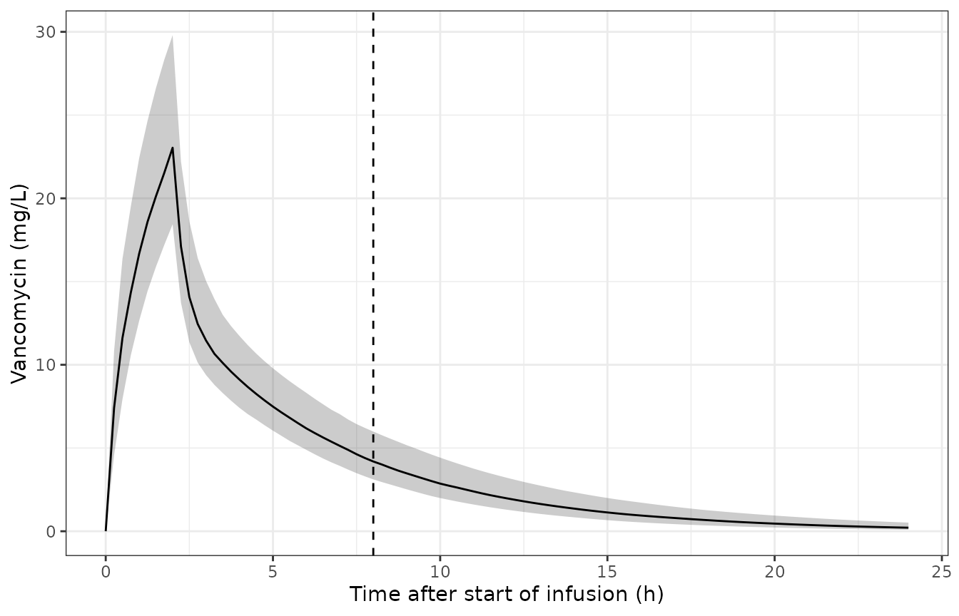
Simulated plasma concentrations after a single 1 g, 2-h IV infusion (median and 10th-90th percentiles; 200 virtual subjects). The paper’s VPC (Figure S2) covers the 0-8 h sampling window.
PKNCA validation
NCA is run on the paper’s sampling schedule (0, 2, 3, 4, 6 and 8 h,
with the pre-dose concentration taken as zero as in Kim 2024 Section
4.2), so the simulated and published NCA see the same design.
AUClast is computed over 0-8 h; Cmax,
AUCinf and the terminal half-life over 0-infinity.
# A subject that fails to solve comes back NA; stop rather than drop it.
stopifnot(!anyNA(sim$Cc))
nca_conc <- sim |>
  filter(time %in% c(0, 2, 3, 4, 6, 8), !is.na(Cc)) |>
  select(id, time, Cc, treatment)
nca_dose <- doses |>
  mutate(dur = 2) |>
  select(id, time, amt, dur, treatment)

conc_obj <- PKNCA::PKNCAconc(nca_conc, Cc ~ time | treatment + id)
dose_obj <- PKNCA::PKNCAdose(
  nca_dose, amt ~ time | treatment + id,
  route = "intravascular", duration = "dur"
)
intervals <- data.frame(
  start = c(0, 0),
  end = c(8, Inf),
  auclast = c(TRUE, FALSE),
  cmax = c(FALSE, TRUE),
  aucinf.obs = c(FALSE, TRUE),
  half.life = c(FALSE, TRUE)
)
nca_res <- PKNCA::pk.nca(PKNCA::PKNCAdata(conc_obj, dose_obj, intervals = intervals))
Comparison against the published NCA
Kim 2024 Table 3 reports the NCA medians;
ncaComparisonTable() pools the simulated side by median
too.
published_nca <- data.frame(
  treatment = "1 g IV over 2 h",
  cmax = 20.8,
  auclast = 73.6,
  aucinf.obs = 97.1,
  half.life = 3.58
)
cmp <- nlmixr2lib::ncaComparisonTable(
  simulated = nca_res,
  reference = published_nca,
  by = "treatment",
  params = c("cmax", "auclast", "aucinf.obs", "half.life"),
  units = c(cmax = "mg/L", auclast = "mg*h/L", aucinf.obs = "mg*h/L", half.life = "h"),
  tolerance_pct = 20
)
knitr::kable(cmp, caption = "Simulated versus published NCA medians (Kim 2024 Table 3).")| NCA parameter | treatment | Reference | Simulated | % diff |
|---|---|---|---|---|
| Cmax (mg/L) | 1 g IV over 2 h | 20.8 | 23 | +10.8% |
| AUC0-∞ (obs) (mg*h/L) | 1 g IV over 2 h | 97.1 | 99 | +1.9% |
| AUClast (mg*h/L) | 1 g IV over 2 h | 73.6 | 74.6 | +1.3% |
| t½ (h) | 1 g IV over 2 h | 3.58 | 3.68 | +2.7% |
The simulated medians agree with the published NCA medians to within the 20% tolerance. The paper’s NCA was run on 12 observed profiles, so a difference of this order is within the sampling noise of a 12-subject median.
Post-hoc parameter summaries
Table 3 also summarises the individual post-hoc parameters of the 12
participants. The same quantities are computed here from each virtual
subject’s parameters: CL and the volumes per kg,
AUCtau = dose/CL, and the distribution and elimination
half-lives from the two-compartment micro-constants.
indiv <- sim |>
  filter(time == 0) |>
  distinct(id, .keep_all = TRUE) |>
  mutate(
    k10 = cl / vc, k12 = q / vc, k21 = q / vp,
    beta_sum = k10 + k12 + k21,
    alpha = (beta_sum + sqrt(beta_sum^2 - 4 * k10 * k21)) / 2,
    beta = (beta_sum - sqrt(beta_sum^2 - 4 * k10 * k21)) / 2,
    cl_kg = cl / WT,
    vc_kg = vc / WT,
    vss_kg = (vc + vp) / WT,
    auctau = 1000 / cl,
    thalf_alpha = log(2) / alpha,
    thalf_beta = log(2) / beta
  )

posthoc_cmp <- indiv |>
  summarise(across(c(cl_kg, vc_kg, vss_kg, auctau, thalf_alpha, thalf_beta), median)) |>
  tidyr::pivot_longer(everything(), names_to = "parameter", values_to = "simulated") |>
  left_join(
    data.frame(
      parameter = c("cl_kg", "vc_kg", "vss_kg", "auctau", "thalf_alpha", "thalf_beta"),
      label = c("CL (L/h/kg)", "VC (L/kg)", "Vss (L/kg)", "AUCtau (mg*h/L)", "t1/2 alpha (h)", "t1/2 beta (h)"),
      published = c(0.131, 0.163, 0.593, 111, 0.259, 3.84)
    ),
    by = "parameter"
  ) |>
  mutate(pct_diff = 100 * (simulated - published) / published)

posthoc_cmp |>
  select(label, published, simulated, pct_diff) |>
  dplyr::rename(
    "Parameter" = label,
    "Kim 2024 Table 3 median" = published,
    "Simulated median" = simulated,
    "% difference" = pct_diff
  ) |>
knitr::kable(digits = 3, caption = "Median individual parameters versus Kim 2024 Table 3 (population PK rows).")| Parameter | Kim 2024 Table 3 median | Simulated median | % difference |
|---|---|---|---|
| CL (L/h/kg) | 0.131 | 0.135 | 3.309 |
| VC (L/kg) | 0.163 | 0.184 | 13.033 |
| Vss (L/kg) | 0.593 | 0.585 | -1.409 |
| AUCtau (mg*h/L) | 111.000 | 105.255 | -5.176 |
| t1/2 alpha (h) | 0.259 | 0.242 | -6.618 |
| t1/2 beta (h) | 3.840 | 3.716 | -3.237 |
At the reference subject (69.45 kg, 38.5 years, 1.80 m^2) the typical
clearance is exactly theta1, so AUCtau for a 1 g dose is
1000 / 8.83 = 113.3 mg h/L, matching the Table 3 post-hoc
mean of 113 mg h/L.
typical <- rxode2::rxSolve(
  rxode2::zeroRe(mod),
  data.frame(
    id = 1, time = c(0, 1), amt = c(1000, 0), rate = c(500, 0),
    evid = c(1L, 0L), cmt = "central", WT = 69.45, AGE = 38.5, BSA = 1.80
  )
) |>
  as.data.frame()
#> ℹ parameter labels from comments will be replaced by 'label()'
#> ℹ omega/sigma items treated as zero: 'etalcl', 'etalvc'

stopifnot(
  # Closed form: the reference-subject clearance is theta1 exactly.
  abs(typical$cl[1] - 8.83) < 1e-8,
  # Structural: a mis-transcribed theta or exponent shifts the whole cohort.
  abs(posthoc_cmp$pct_diff[posthoc_cmp$parameter == "cl_kg"]) < 10,
  abs(posthoc_cmp$pct_diff[posthoc_cmp$parameter == "vss_kg"]) < 10,
  abs(posthoc_cmp$pct_diff[posthoc_cmp$parameter == "thalf_beta"]) < 10
)
Dosing simulations (Figures 2-4)
Kim 2024 Section 4.6 computes the steady-state AUC24 as daily dose / CL for virtual subjects in six age groups, for intermittent doses of 10-30 mg/kg every 6, 8 or 12 h and for continuous infusions of 30-70 mg/kg/day. Because the AUC depends only on the daily dose and CL, every regimen with the same daily dose gives the same AUC distribution (for example 15 mg/kg q6h, 20 mg/kg q8h, 30 mg/kg q12h and a 60 mg/kg/day continuous infusion), which is visible in the paper’s Figures 2 and 3. The virtual cohort below has 200 subjects per age group, with age uniform within the group and weight and height drawn as above.
age_groups <- data.frame(
  age_group = c("20-24", "25-29", "30-34", "35-39", "40-44", "45-49"),
  lo = c(20, 25, 30, 35, 40, 45)
)
n_per_group <- 200
pta_cohort <- bind_rows(lapply(seq_len(nrow(age_groups)), function(i) {
  make_cohort(n_per_group, age_groups$lo[i], age_groups$lo[i] + 5) |>
    mutate(age_group = age_groups$age_group[i])
})) |>
  mutate(id = seq_len(n()))

# Individual CL from the model with IIV: a one-row solve per subject returns
# the algebraic `cl`.
pta_ev <- pta_cohort |>
  mutate(time = 0, amt = 0, evid = 0L, cmt = "central")
pta_cl <- rxode2::rxSolve(mod, pta_ev, keep = "age_group") |>
  as.data.frame() |>
  select(id, age_group, WT, cl)
daily_doses <- c(30, 40, 50, 60, 70, 80, 90, 120)
pta <- pta_cl |>
  tidyr::crossing(daily_mgkg = daily_doses) |>
  mutate(auc24 = daily_mgkg * WT / cl) |>
  group_by(age_group, daily_mgkg) |>
  summarise(
    pta = 100 * mean(auc24 >= 400),
    pct_tox = 100 * sum(auc24 > 600) / max(sum(auc24 >= 400), 1),
    .groups = "drop"
  )

pta |>
  filter(daily_mgkg <= 70) |>
  ggplot(aes(age_group, pta, colour = factor(daily_mgkg), group = factor(daily_mgkg))) +
  geom_point() +
  geom_line() +
  geom_hline(yintercept = 90, linetype = "dashed") +
  labs(x = "Age (years)", y = "Target attainment (%)", colour = "Daily dose (mg/kg)") +
  theme_bw()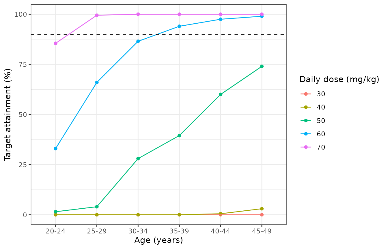
Replicates Figure 3 of Kim 2024 (and, by daily-dose equivalence, Figure 2): probability that the steady-state AUC24 is at least 400 mg h/L, by age group and daily dose.
The table puts the simulated PTA beside the values printed in Kim 2024 Figure 3 (continuous infusion) for the 50 and 60 mg/kg/day rows, which carry the age gradient, and the toxicity percentage (AUC24 > 600 among those with AUC24 >= 400) for 70 mg/kg/day.
published_pta <- data.frame(
  age_group = rep(c("20-24", "25-29", "30-34", "35-39", "40-44", "45-49"), 3),
  quantity = rep(c("PTA, 50 mg/kg/day", "PTA, 60 mg/kg/day", "% AUC > 600, 70 mg/kg/day"), each = 6),
  published = c(
    1, 8, 21, 38, 60, 83,
    41, 72, 87, 95, 100, 100,
    0, 2, 6, 14, 31, 51
  )
)
sim_pta <- bind_rows(
  pta |> filter(daily_mgkg == 50) |> transmute(age_group, quantity = "PTA, 50 mg/kg/day", simulated = pta),
  pta |> filter(daily_mgkg == 60) |> transmute(age_group, quantity = "PTA, 60 mg/kg/day", simulated = pta),
  pta |> filter(daily_mgkg == 70) |> transmute(age_group, quantity = "% AUC > 600, 70 mg/kg/day", simulated = pct_tox)
)
published_pta |>
  left_join(sim_pta, by = c("age_group", "quantity")) |>
  tidyr::pivot_longer(c(published, simulated), names_to = "source") |>
  tidyr::pivot_wider(names_from = age_group, values_from = value) |>
  dplyr::rename("Quantity" = quantity, "Source" = source) |>
knitr::kable(digits = 0, caption = "Target attainment (%) by age group: Kim 2024 Figure 3 versus this simulation.")| Quantity | Source | 20-24 | 25-29 | 30-34 | 35-39 | 40-44 | 45-49 |
|---|---|---|---|---|---|---|---|
| PTA, 50 mg/kg/day | published | 1 | 8 | 21 | 38 | 60 | 83 |
| PTA, 50 mg/kg/day | simulated | 2 | 4 | 28 | 40 | 60 | 74 |
| PTA, 60 mg/kg/day | published | 41 | 72 | 87 | 95 | 100 | 100 |
| PTA, 60 mg/kg/day | simulated | 33 | 66 | 86 | 94 | 98 | 99 |
| % AUC > 600, 70 mg/kg/day | published | 0 | 2 | 6 | 14 | 31 | 51 |
| % AUC > 600, 70 mg/kg/day | simulated | 0 | 0 | 6 | 16 | 28 | 42 |
The simulation reproduces the paper’s pattern: PTA rises steeply with
age at a fixed mg/kg dose, because clearance falls with age (exponent
-0.377) while the small IIV on CL (7.98% CV) and the weak net weight
dependence of the AUC (WT^(1 - 1.28)) leave little
between-subject spread. The age gradient in the simulation is close to
the published one; the exact percentages depend on the weight and age
distributions within each group, which the paper describes only as
“log-normally distributed random variables across a demographic
range”.
AUC versus trough (Figure 4)
Figure 4 relates the steady-state AUC24 to the trough concentration for the intermittent regimens. The model is linear, so each subject is solved once per dosing interval at 10 mg/kg and the trough and AUC are scaled to the other doses. The paper does not state the infusion duration used for the intermittent regimens; 1 h is assumed here.
trough_ev <- bind_rows(lapply(c(6, 8, 12), function(tau) {
  base <- pta_cohort |>
    mutate(id = id + 10000 * tau, tau = tau)
  bind_rows(
    base |> mutate(time = 0, amt = 10 * WT, rate = 10 * WT, ii = tau, ss = 1L, evid = 1L, cmt = "central"),
    base |> mutate(time = tau, amt = 0, rate = 0, ii = 0, ss = 0L, evid = 0L, cmt = "central")
  )
})) |>
  arrange(id, time, desc(evid))

# steady-state searches for long-half-life subjects exceed the default step budget
trough_sim <- rxode2::rxSolve(mod, trough_ev, keep = c("age_group", "tau"), maxsteps = 1e6) |>
  as.data.frame() |>
  filter(time == tau) |>
  mutate(auc24_10 = 10 * WT * (24 / tau) / cl, trough_10 = Cc)

trough_all <- trough_sim |>
  tidyr::crossing(dose_mgkg = c(10, 15, 20, 25, 30)) |>
  mutate(
    auc24 = auc24_10 * dose_mgkg / 10,
    trough = trough_10 * dose_mgkg / 10,
    interval = paste0("q", tau, "h")
  )
ggplot(trough_all, aes(trough, auc24, colour = factor(dose_mgkg))) +
  geom_point(size = 0.4, alpha = 0.4) +
  annotate("rect", xmin = 15, xmax = 20, ymin = 400, ymax = 600, fill = NA, colour = "black") +
  facet_grid(interval ~ age_group) +
  labs(x = "Trough concentration (mg/L)", y = "AUC24 (mg*h/L)", colour = "Dose (mg/kg)") +
  theme_bw()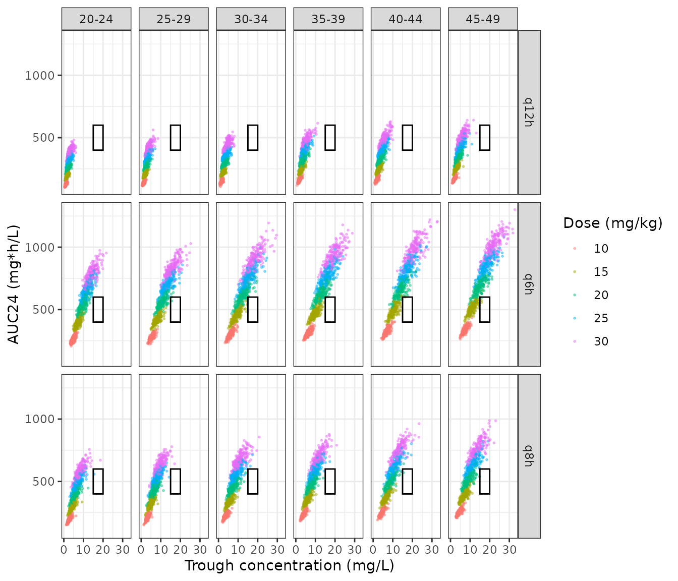
Replicates Figure 4 of Kim 2024: steady-state AUC24 versus trough concentration for intermittent dosing (1-h infusion assumed).
trough_all |>
  group_by(interval, age_group) |>
  summarise(slope = unname(stats::coef(stats::lm(auc24 ~ trough))[2]), .groups = "drop") |>
  tidyr::pivot_wider(names_from = age_group, values_from = slope) |>
  dplyr::rename("Interval" = interval) |>
knitr::kable(digits = 0, caption = "Slope of AUC24 on trough (mg h/L per mg/L). Kim 2024 Figure 4 prints slopes of 29-31 (q6h), 35-38 (q8h) and 47-55 (q12h).")| Interval | 20-24 | 25-29 | 30-34 | 35-39 | 40-44 | 45-49 |
|---|---|---|---|---|---|---|
| q12h | 75 | 70 | 64 | 60 | 60 | 59 |
| q6h | 49 | 45 | 42 | 42 | 41 | 41 |
| q8h | 52 | 52 | 47 | 49 | 47 | 45 |
The qualitative finding of the paper is reproduced: on q6h and q8h dosing a trough of 15-20 mg/L corresponds to an AUC24 above 600 mg h/L, while q12h regimens reach AUC24 >= 400 mg h/L at troughs below 15 mg/L. The simulated slopes are, however, roughly 40-50% steeper than the slopes printed in Figure 4 (the simulated troughs are lower for a given AUC24), and the printed intercepts (96-150 mg h/L) are higher than the simulated ones. Varying the assumed infusion duration from 0.5 to 3 h changes the simulated slopes by less than 15%, so the infusion duration does not account for the gap. The paper does not report the remaining settings of the Figure 4 simulation (the covariate distributions, and how the trough was computed), so the difference is recorded here rather than resolved. The AUC24-based target attainment of Figures 2 and 3, which does not involve the trough, is reproduced closely (table above).
Assumptions and deviations
-
IIV scale. Table 2 reports IIV as a percentage
without stating whether it is a CV or
sqrt(omega^2). It is converted withomega^2 = log(CV^2 + 1). For CL (7.98%) the two readings agree to four digits; for the fixed V1 IIV (47.4%) they give 0.203 versus 0.225. - IIV on Q and V2. Section 2.2 says the IIV on Q and V2 fell “to nearly 0” once weight and BSA entered the model, and Table 2 lists no IIV for either, so neither parameter carries an eta.
- Virtual-cohort covariates. The paper gives Table 1 summaries only. Weight is drawn log-normally (median 69.5 kg, CV 18%), height normally (mean 170 cm, SD 7.1 cm), both truncated to the observed range, and BSA is computed by the DuBois formula. For the age-group simulations, age is uniform within each 5-year group. The paper describes its simulation covariates only as log-normally distributed “across a demographic range”.
- Cohort size. The paper simulated 2000 subjects (intermittent) and 1000 subjects (continuous); 200 per age group are used here.
- Intermittent infusion duration. Not stated for Figure 4; 1 h is assumed. The AUC values (Figures 2-3) do not depend on it; the troughs do.
-
Table 3 labels. The
ClastandTlastrows of Table 3 carry swapped units (Clastin h,Tlastin mg/L); from the values (Tlast about 8 h, matching the last sampling time) the labels, not the numbers, are swapped. Neither row is used here. - Table S1 title. The supplement titles the base-model table “meropenem”; the values are the vancomycin base model described in Section 2.2.