Model and source
- Citation: Niu C-H, Xu H, Gao L-L, Nie Y-M, Xing L-P, Yu L-P, Wu S-L, Wang Y. Population Pharmacokinetics of Caspofungin and Dosing Optimization in Children With Allogeneic Hematopoietic Stem Cell Transplantation. Front Pharmacol. 2020;11:184. doi:10.3389/fphar.2020.00184.
- Description: One-compartment population PK model with first-order elimination and proportional residual error for once-daily 1-hour intravenous caspofungin infusions (70 mg/m^2 loading dose on day 1, then 50 mg/m^2 daily) in children aged 0.6-14 years undergoing allogeneic hematopoietic stem cell transplantation (Niu 2020). Clearance scales with body surface area (power 0.89) and with the natural log of aspartate aminotransferase (power -0.23 on ln(AST), centred on ln(AST) = 3.38); volume of distribution is proportional to body surface area. Both are centred on BSA = 0.79 m^2. Exponential inter-individual variability on CL and Vd.
- Article: Front Pharmacol 2020;11:184
Population
Niu 2020 enrolled 48 children (31 male, 17 female) undergoing allogeneic hematopoietic stem cell transplantation at Wuhan Children’s Hospital, China, between July 2017 and March 2019. Caspofungin was given as antifungal prophylaxis: 70 mg/m^2 on day 1, then 50 mg/m^2 once daily, each as a 1-hour intravenous infusion. Table 1 of the paper gives the baseline demographics. Age was 0.61-14 years (mean 6.58, median 6.2), body weight 7.5-54 kg (mean 21.7), and body surface area (Mosteller) 0.38-1.50 m^2 (mean 0.80). Median AST was 26 U/L. Thirty-seven children had normal hepatic function (AST <= 40 U/L), nine had mild dysfunction (40-120 U/L) and two had severe dysfunction (> 120 U/L).
Sampling was opportunistic at steady state: 139 concentrations, 2.9 per patient, mean 17.5 h after the last dose. The concentrations were 4.5-17.4 mg/L by HPLC-UV (LLOQ 0.6 mg/L). The model was fitted in Phoenix NLME 8.1.
The same information is available programmatically via
readModelDb("Niu_2020_caspofungin")()$population.
Source trace
Each ini() entry in
inst/modeldb/specificDrugs/Niu_2020_caspofungin.R has an
in-file comment giving its origin. The table below collects them.
| Equation / parameter | Value | Source location |
|---|---|---|
lcl |
log(0.14 L/h) | Table 3, theta CL = 0.14 (SE 8.50%); final-model CL equation (Results, “Population Pharmacokinetic Model Building”) |
lvc |
log(1.36 L) | Table 3, theta Vd = 1.36 (SE 15.58%); final-model Vd equation |
e_bsa_cl |
0.89 | Table 3, theta 1 = 0.89 (SE 11.36%); CL equation
(BSA/0.79)^0.89
|
e_ast_cl |
-0.23 | Table 3, theta 2 = -0.23 (SE 39.13%); CL equation
(lnAST/3.38)^-0.23
|
e_bsa_vc |
1 (fixed) | Vd equation 1.36 x (BSA/0.79): exponent 1, not in Table
3 |
etalcl |
0.333^2 = 0.1109 | Table 3, omega CL = 33.3%; the footnote defines omega as the “square root of inter-individual variance” |
etalvc |
0.329^2 = 0.1082 | Table 3, omega Vd = 32.9% |
propSd |
0.266 | Table 3, residual variability sigma = 26.6% (proportional; Results) |
| One-compartment, first-order elimination | n/a | Results, “Population Pharmacokinetic Model Building” |
| 1-h IV infusion, 70 mg/m^2 then 50 mg/m^2 daily | n/a | Methods, “Study Design” |
| BSA = sqrt(height x weight / 3600) | n/a | Methods, Mosteller equation |
Virtual cohort
The individual data are not public. Table 4 of the paper reports probability of target attainment (PTA) for infants, children aged 2-11 years and adolescents aged 12-14 years, so the virtual cohort has one arm for each of those three age groups, with 150 subjects per arm. The paper does not give BSA or AST distributions by age group. BSA is therefore drawn uniformly over a band for each group, and the bands together span the observed 0.38-1.50 m^2. AST is drawn log-normally around the cohort median of 26 U/L and truncated at 120 U/L. The paper’s PTA simulations excluded the two children with severe hepatic dysfunction, and this truncation does the same. Each subject receives 70 mg/m^2 on day 1 and then 50 mg/m^2 daily for 7 days, all as 1-h infusions.
set.seed(20200302L)
rxode2::rxSetSeed(20200302L)

n_per_arm <- 150L
tau <- 24
n_doses <- 7L

arms <- tibble::tribble(
  ~agegroup                    , ~bsa_lo , ~bsa_hi ,
  "Infants"                    ,    0.38 ,    0.55 ,
  "Children (2-11 years)"      ,    0.55 ,    1.20 ,
  "Adolescents (12-14 years)"  ,    1.10 ,    1.50
)

subjects <- arms |>
  dplyr::slice(rep(seq_len(dplyr::n()), each = n_per_arm)) |>
  dplyr::mutate(
    id = dplyr::row_number(),
    BSA = stats::runif(dplyr::n(), bsa_lo, bsa_hi),
    AST = pmin(pmax(exp(stats::rnorm(dplyr::n(), log(26), 0.45)), 10), 120)
  ) |>
  dplyr::select(id, agegroup, BSA, AST)

dose_rows <- subjects |>
  tidyr::crossing(dose_no = seq_len(n_doses)) |>
  dplyr::mutate(
    time = (dose_no - 1) * tau,
    amt = ifelse(dose_no == 1, 70, 50) * BSA,
    rate = amt / 1,
    evid = 1L,
    cmt = "central"
  ) |>
  dplyr::select(-dose_no)

obs_times <- sort(unique(c(seq(0, 24, by = 0.5), seq(144, 168, by = 0.5))))
obs_rows <- subjects |>
  tidyr::crossing(time = obs_times) |>
  dplyr::mutate(amt = 0, rate = 0, evid = 0L, cmt = "central")

events <- dplyr::bind_rows(dose_rows, obs_rows) |>
  dplyr::arrange(id, time, dplyr::desc(evid))
Simulation
mod <- readModelDb("Niu_2020_caspofungin")
sim <- rxode2::rxSolve(
  mod,
  events = events,
  keep = c("agegroup", "BSA", "AST")
) |>
  as.data.frame()
#> ℹ parameter labels from comments will be replaced by 'label()'
Structural checks against the text
The Results state that the Bayesian BSA-normalised estimates were CL = 0.19 +/- 0.04 L/m^2/h and Vd = 1.72 +/- 0.01 L/m^2. The typical Vd per m^2 at the reference BSA is 1.36 / 0.79 = 1.72 L/m^2, which matches the text exactly. The typical CL per m^2 is 0.14 / 0.79 = 0.177 L/m^2/h. The paper’s 0.19 is a cohort mean of individual estimates, so it includes the log-normal mean shift exp(omega^2 / 2) = 1.057. The same summary over the simulated cohort is therefore the like-for-like comparison.
typ_vd_per_m2 <- 1.36 / 0.79
indiv <- sim |>
  dplyr::distinct(id, agegroup, BSA, cl, vc)
cl_per_m2 <- mean(indiv$cl / indiv$BSA)

knitr::kable(
  data.frame(
    Quantity = c("Typical Vd / BSA (L/m^2)", "Cohort mean CL / BSA (L/m^2/h)"),
    Model = c(typ_vd_per_m2, cl_per_m2),
    Paper = c(1.72, 0.19)
  ),
  digits = 3,
  caption = "BSA-normalised parameters compared with Niu 2020 Results."
)| Quantity | Model | Paper |
|---|---|---|
| Typical Vd / BSA (L/m^2) | 1.722 | 1.72 |
| Cohort mean CL / BSA (L/m^2/h) | 0.188 | 0.19 |
Replicate published figures
Figure 1 – steady-state concentrations against time since the last dose
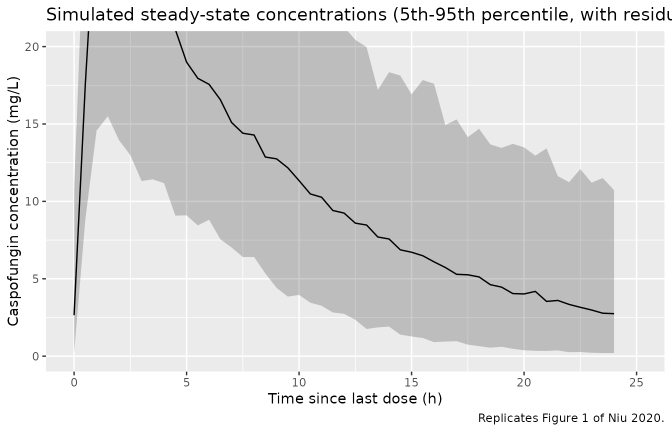
Figure 1 of Niu 2020 plots the 139 observed concentrations, sampled 7-23 h after the last dose, against time since that dose. The figure below shows the simulated steady-state (day 7) median and 5th-95th percentile band over the same window.
ss_start <- (n_doses - 1) * tau
fig1 <- sim |>
  dplyr::filter(time >= ss_start, time <= ss_start + tau) |>
  dplyr::mutate(tad = time - ss_start) |>
  dplyr::group_by(tad) |>
  dplyr::summarise(
    q05 = stats::quantile(sim, 0.05),
    q50 = stats::quantile(sim, 0.50),
    q95 = stats::quantile(sim, 0.95),
    .groups = "drop"
  )

ggplot(fig1, aes(tad, q50)) +
  geom_ribbon(aes(ymin = q05, ymax = q95), alpha = 0.25) +
  geom_line() +
  coord_cartesian(xlim = c(0, 25), ylim = c(0, 20)) +
  labs(
    x = "Time since last dose (h)",
    y = "Caspofungin concentration (mg/L)",
    title = "Simulated steady-state concentrations (5th-95th percentile, with residual error)",
    caption = "Replicates Figure 1 of Niu 2020."
  )
PKNCA validation
NCA is run on the day-1 loading-dose interval (0-24 h) and on the day-7 maintenance interval (144-168 h).
conc_df <- sim |>
  dplyr::filter(!is.na(Cc)) |>
  dplyr::select(id, time, Cc, agegroup)
dose_df <- events |>
  dplyr::filter(evid == 1L) |>
  dplyr::select(id, time, amt, agegroup)

conc_obj <- PKNCA::PKNCAconc(conc_df, Cc ~ time | agegroup + id, concu = "mg/L", timeu = "hr")
dose_obj <- PKNCA::PKNCAdose(dose_df, amt ~ time | agegroup + id, doseu = "mg")

intervals <- data.frame(
  start = c(0, ss_start),
  end = c(tau, ss_start + tau),
  cmax = TRUE,
  cmin = TRUE,
  auclast = TRUE
)
nca_res <- PKNCA::pk.nca(PKNCA::PKNCAdata(conc_obj, dose_obj, intervals = intervals))

nca_df <- as.data.frame(nca_res) |>
  dplyr::mutate(window = ifelse(start == 0, "Day 1 (70 mg/m^2)", "Day 7 (50 mg/m^2)"))

nca_df |>
  dplyr::filter(PPTESTCD %in% c("cmax", "cmin", "auclast")) |>
  dplyr::group_by(window, agegroup, PPTESTCD) |>
  dplyr::summarise(median = stats::median(PPORRES), .groups = "drop") |>
  tidyr::pivot_wider(names_from = PPTESTCD, values_from = median) |>
  dplyr::rename(
    "Interval" = window,
    "Age group" = agegroup,
    "Cmax (mg/L)" = cmax,
    "Cmin (mg/L)" = cmin,
    "AUC0-24 (mg*h/L)" = auclast
  ) |>
knitr::kable(digits = 1, caption = "Simulated NCA (median) by interval and age group.")| Interval | Age group | AUC0-24 (mg*h/L) | Cmax (mg/L) | Cmin (mg/L) |
|---|---|---|---|---|
| Day 1 (70 mg/m^2) | Adolescents (12-14 years) | 370.7 | 37.5 | 0.0 |
| Day 1 (70 mg/m^2) | Children (2-11 years) | 349.6 | 38.2 | 0.0 |
| Day 1 (70 mg/m^2) | Infants | 319.9 | 37.1 | 0.0 |
| Day 7 (50 mg/m^2) | Adolescents (12-14 years) | 299.2 | 31.0 | 3.2 |
| Day 7 (50 mg/m^2) | Children (2-11 years) | 288.7 | 31.0 | 2.9 |
| Day 7 (50 mg/m^2) | Infants | 253.3 | 29.6 | 2.4 |
Comparison against the published AUC24
The paper’s “Clinical Outcomes” section reports AUC24 for 44 successful and 4 failed prophylaxis cases, with separate values for the loading and maintenance doses. Successful cases had 394.93 and 300.37 mgh/L, and failed cases 352.08 and 247.71 mgh/L. The case-weighted cohort means are compared below with the mean simulated AUC0-24 on day 1 and day 7.
ref_auc <- data.frame(
  window = c("Day 1 (70 mg/m^2)", "Day 7 (50 mg/m^2)"),
  auclast = c((44 * 394.93 + 4 * 352.08) / 48, (44 * 300.37 + 4 * 247.71) / 48)
)
sim_auc <- nca_df |>
  dplyr::filter(PPTESTCD == "auclast") |>
  dplyr::group_by(window) |>
  dplyr::summarise(PPTESTCD = "auclast", PPORRES = mean(PPORRES), .groups = "drop")

cmp <- nlmixr2lib::ncaComparisonTable(
  simulated = sim_auc,
  reference = ref_auc,
  by = "window",
  units = c(auclast = "mg*h/L")
)
knitr::kable(cmp, caption = "Mean AUC0-24: simulation vs Niu 2020 Clinical Outcomes.")| NCA parameter | window | Reference | Simulated | % diff |
|---|---|---|---|---|
| AUClast (mg*h/L) | Day 1 (70 mg/m^2) | 391 | 358 | -8.5% |
| AUClast (mg*h/L) | Day 7 (50 mg/m^2) | 296 | 298 | +0.7% |
sim_vs_ref <- dplyr::inner_join(sim_auc, ref_auc, by = "window")
stopifnot(all(abs(sim_vs_ref$PPORRES / sim_vs_ref$auclast - 1) < 0.15))
Probability of target attainment (Table 4)
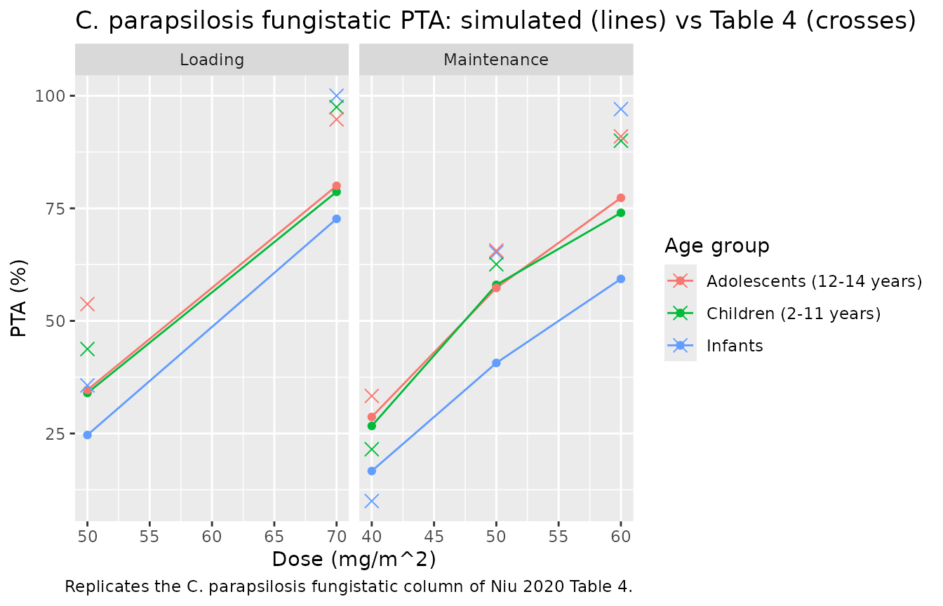
Table 4 gives PTA for AUC24/MIC targets at the MIC90 of each species. For C. albicans and C. glabrata every regimen reaches 100%. The discriminating column is the C. parapsilosis fungistatic target: AUC24/MIC >= 559 at an MIC of 0.5 mg/L, which is AUC24 >= 279.5 mg*h/L. The model is linear, so AUC scales in proportion to dose. The alternative regimens are therefore obtained by rescaling the simulated day-1 AUC (for the loading-dose rows) and the day-7 AUC (for the maintenance rows). By day 7 the loading dose contributes nothing measurable, because six days is more than 20 half-lives. PTA here is computed from the individual AUC0-24 without residual error.
auc_ind <- nca_df |>
  dplyr::filter(PPTESTCD == "auclast") |>
  dplyr::select(id, agegroup, window, auc = PPORRES)

regimens <- tibble::tribble(
  ~phase         , ~dose ,
  "Loading"      ,    50 ,
  "Loading"      ,    70 ,
  "Maintenance"  ,    40 ,
  "Maintenance"  ,    50 ,
  "Maintenance"  ,    60
)

pta <- regimens |>
  dplyr::mutate(window = ifelse(phase == "Loading", "Day 1 (70 mg/m^2)", "Day 7 (50 mg/m^2)"),
                base_dose = ifelse(phase == "Loading", 70, 50)) |>
  dplyr::inner_join(auc_ind, by = "window", relationship = "many-to-many") |>
  dplyr::mutate(auc_scaled = auc * dose / base_dose) |>
  dplyr::group_by(phase, dose, agegroup) |>
  dplyr::summarise(pta_sim = 100 * mean(auc_scaled / 0.5 >= 559), .groups = "drop")

pub_pta <- tibble::tribble(
  ~phase         , ~dose , ~agegroup                    , ~pta_pub ,
  "Loading"      ,    50 , "Infants"                    ,    35.68 ,
  "Loading"      ,    70 , "Infants"                    ,   100    ,
  "Loading"      ,    50 , "Children (2-11 years)"      ,    43.75 ,
  "Loading"      ,    70 , "Children (2-11 years)"      ,    97.48 ,
  "Loading"      ,    50 , "Adolescents (12-14 years)"  ,    53.73 ,
  "Loading"      ,    70 , "Adolescents (12-14 years)"  ,    94.75 ,
  "Maintenance"  ,    40 , "Infants"                    ,     9.99 ,
  "Maintenance"  ,    50 , "Infants"                    ,    65.21 ,
  "Maintenance"  ,    60 , "Infants"                    ,    97.03 ,
  "Maintenance"  ,    40 , "Children (2-11 years)"      ,    21.50 ,
  "Maintenance"  ,    50 , "Children (2-11 years)"      ,    62.57 ,
  "Maintenance"  ,    60 , "Children (2-11 years)"      ,    90.01 ,
  "Maintenance"  ,    40 , "Adolescents (12-14 years)"  ,    33.34 ,
  "Maintenance"  ,    50 , "Adolescents (12-14 years)"  ,    65.63 ,
  "Maintenance"  ,    60 , "Adolescents (12-14 years)"  ,    90.98
)

pta_cmp <- dplyr::inner_join(pub_pta, pta, by = c("phase", "dose", "agegroup"))
pta_cmp |>
  dplyr::rename(
    "Phase" = phase,
    "Dose (mg/m^2)" = dose,
    "Age group" = agegroup,
    "PTA, Niu 2020 Table 4 (%)" = pta_pub,
    "PTA, simulated (%)" = pta_sim
  ) |>
knitr::kable(digits = 1, caption = "C. parapsilosis fungistatic PTA (AUC24/MIC >= 559, MIC 0.5 mg/L).")| Phase | Dose (mg/m^2) | Age group | PTA, Niu 2020 Table 4 (%) | PTA, simulated (%) |
|---|---|---|---|---|
| Loading | 50 | Infants | 35.7 | 24.7 |
| Loading | 70 | Infants | 100.0 | 72.7 |
| Loading | 50 | Children (2-11 years) | 43.8 | 34.0 |
| Loading | 70 | Children (2-11 years) | 97.5 | 78.7 |
| Loading | 50 | Adolescents (12-14 years) | 53.7 | 34.7 |
| Loading | 70 | Adolescents (12-14 years) | 94.8 | 80.0 |
| Maintenance | 40 | Infants | 10.0 | 16.7 |
| Maintenance | 50 | Infants | 65.2 | 40.7 |
| Maintenance | 60 | Infants | 97.0 | 59.3 |
| Maintenance | 40 | Children (2-11 years) | 21.5 | 26.7 |
| Maintenance | 50 | Children (2-11 years) | 62.6 | 58.0 |
| Maintenance | 60 | Children (2-11 years) | 90.0 | 74.0 |
| Maintenance | 40 | Adolescents (12-14 years) | 33.3 | 28.7 |
| Maintenance | 50 | Adolescents (12-14 years) | 65.6 | 57.3 |
| Maintenance | 60 | Adolescents (12-14 years) | 91.0 | 77.3 |
ggplot(pta_cmp, aes(dose, pta_sim, colour = agegroup)) +
  geom_line() +
  geom_point() +
  geom_point(aes(y = pta_pub), shape = 4, size = 3) +
  facet_wrap(~phase, scales = "free_x") +
  labs(
    x = "Dose (mg/m^2)",
    y = "PTA (%)",
    colour = "Age group",
    title = "C. parapsilosis fungistatic PTA: simulated (lines) vs Table 4 (crosses)",
    caption = "Replicates the C. parapsilosis fungistatic column of Niu 2020 Table 4."
  )
# The simulated PTA must rise with dose within every phase and age group.
monotone <- pta_cmp |>
  dplyr::arrange(phase, agegroup, dose) |>
  dplyr::group_by(phase, agegroup) |>
  dplyr::summarise(ok = all(diff(pta_sim) > 0), .groups = "drop")
stopifnot(all(monotone$ok))
The simulated PTA rises with dose, as Table 4 does. For children and adolescents on 40 and 50 mg/m^2 maintenance it lies within about 10 percentage points of the published values. The simulated dose-response is flatter, though. Table 4 goes from 10-33% at 40 mg/m^2 to 90-97% at 60 mg/m^2, but the simulation goes from 17-29% to 59-77%. Loading-dose PTA at 70 mg/m^2 is 73-80% simulated against 95-100% published.
A step that steep implies a much narrower spread of AUC24 across subjects than the final model’s IIV on CL (33%) produces. The model’s spread is consistent with the paper’s own observed data: the “Clinical Outcomes” AUC24 SDs are 91 and 88 mgh/L on means of about 390 and 300 mgh/L, which are CVs of 23-29%. The cohort means themselves agree (the comparison table above).
The simulation also gives infants lower PTA than older children. With BSA-based dosing, AUC is proportional to BSA^(1 - 0.89) = BSA^0.11, so the smallest children have the lowest exposure. Table 4 does not show this ordering. The paper does not describe how its Monte Carlo cohort was built (covariates, variability terms, number of subjects), so these differences are reported here rather than tuned away. The final model reproduces the paper’s structural summaries (BSA-normalised CL and Vd) and its observed cohort-mean AUC24.
Assumptions and deviations
-
Final-model equation vs Table 3 footnote. The Table
3 footnote describes theta 1 as the “exponent for BSA as covariate for
Vd”. The printed final-model equations put the 0.89 exponent on CL and
give Vd = 1.36 x (BSA/0.79), exponent 1. The text also says that BSA and
AST were retained “as significant impacts on caspofungin clearance”, and
Table 2 screened covariates on CL only. The equations are used:
e_bsa_cl = 0.89, ande_bsa_vcis fixed at 1. -
ln(AST) covariate form. The CL factor is
(ln(AST) / 3.38)^-0.23, which follows the printed equation exactly. The reference is AST = exp(3.38), about 29.4 U/L. The form is undefined for AST <= 1 U/L. - IIV scale. Table 3 reports omega as a percentage. The footnote defines it as the square root of the inter-individual variance, so the variances are 0.329^2 and 0.333^2. No CL-Vd covariance was reported, so the two etas are independent.
-
Residual error. The paper uses a “scale”
(proportional) residual model with sigma = 26.6%, encoded as
propSd = 0.266. - Covariate distributions. The BSA bands for each age group and the log-normal AST distribution (median 26 U/L, SD 0.45 on the log scale, truncated to 10-120 U/L) are assumptions, because the paper gives only whole-cohort summaries (Table 1). The age cut for “infants” is not stated; children under 2 years are assumed.
- Observed AUC24. The paper describes its AUC24 summaries as “median +/- standard deviation” but compares them with a t-test, so they are treated as means. The day of the maintenance AUC24 is not stated, so it is compared against simulated steady state (day 7).
- No supplement or erratum. Europe PMC listed no supplementary material and no correction notice for the article as of 2026-09-25.