Nivolumab + ipilimumab exposure-response in hepatocellular carcinoma (Sangro 2023)
Source:vignettes/articles/Sangro_2023_nivolumab_ipilimumab_hcc.Rmd
Sangro_2023_nivolumab_ipilimumab_hcc.RmdSource and models
- Citation: Sangro B, Yau T, El-Khoueiry AB, Kudo M, Shen Y, Tschaika M, Roy A, Feng Y, Gao L, Aras U. Exposure-response analysis for nivolumab plus ipilimumab combination therapy in patients with advanced hepatocellular carcinoma (CheckMate 040). Clin Transl Sci. 2023;16(8):1445-1457. doi:10.1111/cts.13544. PMCID PMC10432868. Coefficients are transcribed from Table 2. The first-dose exposures came from updated versions of the population PK models packaged as modellib(‘Bajaj_2017_nivolumab’) and modellib(‘Sanghavi_2020_ipilimumab’).
- Article (open access): https://doi.org/10.1111/cts.13544
- PubMed Central: https://www.ncbi.nlm.nih.gov/pmc/articles/PMC10432868/
- Supporting Information (Data S1; Tables S1-S3 and Figures S1-S3): distributed with the open-access article.
Sangro 2023 is an exposure-response analysis of CheckMate 040 in sorafenib-experienced patients with advanced hepatocellular carcinoma (HCC). It fits two separate efficacy models, and this package carries each as its own file:
| Model file | Endpoint | Source |
|---|---|---|
Sangro_2023_nivolumab_ipilimumab_orr |
Objective tumor response (OTR) by blinded independent central review, logistic regression | Table 2 |
Sangro_2023_nivolumab_ipilimumab_os |
Overall survival, Cox proportional hazards (relative hazard only) | Table 3 |
Both models are driven by the model-predicted average serum
concentration over the first dosing interval (Cavg1) of
nivolumab (CAV_NIVOLUMAB) and of ipilimumab
(CAV_IPILIMUMAB). The authors derived Cavg1 from updated
versions of two population PK models that this package also carries,
Bajaj_2017_nivolumab and
Sanghavi_2020_ipilimumab. Those updated refits are not
reported, so this vignette regenerates Cavg1 from the published
originals and compares the result with Table S2.
The safety analysis (hepatic treatment-related and immune-mediated adverse events, Table 4) is descriptive incidence by arm with no fitted model, so there is nothing to encode from it.
Population
The analysis population is 328 sorafenib-experienced adults from CheckMate 040 (Sangro 2023 Table 1): 182 received nivolumab monotherapy 0.1-10 mg/kg every 2 weeks (cohorts 1 and 2) and 146 received nivolumab plus ipilimumab in cohort 4:
- Arm A: nivolumab 1 mg/kg + ipilimumab 3 mg/kg every 3 weeks for four doses, then nivolumab 240 mg every 2 weeks (n = 49).
- Arm B: nivolumab 3 mg/kg + ipilimumab 1 mg/kg every 3 weeks for four doses, then nivolumab 240 mg every 2 weeks (n = 49).
- Arm C: nivolumab 3 mg/kg every 2 weeks + ipilimumab 1 mg/kg every 6 weeks (n = 48).
Median age was 62 years (18-83), median weight 67 kg (38-130), and 21% were female. 46% were Asian and 41% White. ECOG performance status was 0 in 60% and 1 in 40%. Child-Pugh class was A in 98%, and 86% had extrahepatic spread or vascular invasion. HCC etiology was hepatitis B in 41%, hepatitis C in 20% and uninfected in 37%.
Source trace
| Quantity | Value | Source |
|---|---|---|
OTR intercept logit_ref
|
-1.419 (OR 0.242) | Table 2, Intercept |
OTR nivolumab Cavg1 slope e_cav_nivolumab_logit
|
-0.00841 per ug/mL (OR 0.9916) | Table 2, Nivolumab Cavg1 |
OTR ipilimumab log-Cavg1 slope
e_cav_ipilimumab_logit
|
0.3712 (OR 1.45) | Table 2, Log-transformed ipilimumab Cavg1 |
| OTR model form: linear nivolumab, log ipilimumab, no other covariate | – | Results, “Objective tumor response” paragraph 2 |
OS nivolumab log-Cavg1 e_cav_nivolumab_haz
|
0.07747 (HR 1.081) | Table 3 |
OS ipilimumab log-Cavg1 e_cav_ipilimumab_haz
|
-0.1539 (HR 0.8574) | Table 3 |
OS ECOG > 0 e_ecog_ge1_haz
|
0.4444 (HR 1.56) | Table 3 |
OS baseline nivolumab CL e_cli_haz
|
0.05068 per mL/h (HR 1.052) | Table 3 and its note |
OS log LDH/ULN e_ldhr_haz
|
0.7962 (HR 2.217) | Table 3 and its note |
| Cavg1 definition (first-dose time-averaged concentration) | – | Methods, “Pharmacokinetic assessments” |
| Arm geometric-mean Cavg1 | Table S2; Results text for ipilimumab | Table S2; Results “Nivolumab and ipilimumab exposures” |
| Observed OTR by group | Table S2 | Table S2 |
| Reference exposure for Figures 2 and 3 (nivolumab Cavg1 25 ug/mL, no ipilimumab) | – | Figure 2 and Figure 3 captions |
Placeholder addSd_prob_orr_central
|
0.001 (fixed) | not from source |
Coefficient check against the printed odds and hazard ratios
Every coefficient is printed together with its odds or hazard ratio,
so exp(coefficient) must reproduce the printed ratio to its
printed precision.
ini_orr <- rxode2::rxode2(mod_orr)$iniDf
ini_os <- rxode2::rxode2(mod_os)$iniDf
coef_of <- function(ini, nm) ini$est[ini$name == nm]

coef_tbl <- tibble::tribble(
  ~model, ~parameter, ~printed_ratio,
  "OTR", "logit_ref", 0.242,
  "OTR", "e_cav_nivolumab_logit", 0.9916,
  "OTR", "e_cav_ipilimumab_logit", 1.45,
  "OS", "e_cav_nivolumab_haz", 1.081,
  "OS", "e_cav_ipilimumab_haz", 0.8574,
  "OS", "e_ecog_ge1_haz", 1.56,
  "OS", "e_cli_haz", 1.052,
  "OS", "e_ldhr_haz", 2.217
) |>
  mutate(
    estimate = mapply(
      function(m, p) coef_of(if (m == "OTR") ini_orr else ini_os, p),
      model,
      parameter
    ),
    exp_estimate = exp(estimate),
    pct_diff = 100 * (exp_estimate - printed_ratio) / printed_ratio
  )

coef_tbl |>
  mutate(across(c(exp_estimate, pct_diff), \(x) signif(x, 4))) |>
  dplyr::rename(
    Model = model,
    Parameter = parameter,
    Estimate = estimate,
    "exp(estimate)" = exp_estimate,
    "Printed ratio" = printed_ratio,
    "% difference" = pct_diff
  ) |>
knitr::kable(caption = "exp(coefficient) against the odds / hazard ratios printed in Sangro 2023 Tables 2 and 3.")| Model | Parameter | Printed ratio | Estimate | exp(estimate) | % difference |
|---|---|---|---|---|---|
| OTR | logit_ref | 0.2420 | -1.41900 | 0.2420 | -0.018240 |
| OTR | e_cav_nivolumab_logit | 0.9916 | -0.00841 | 0.9916 | 0.002548 |
| OTR | e_cav_ipilimumab_logit | 1.4500 | 0.37120 | 1.4490 | -0.036350 |
| OS | e_cav_nivolumab_haz | 1.0810 | 0.07747 | 1.0810 | -0.041650 |
| OS | e_cav_ipilimumab_haz | 0.8574 | -0.15390 | 0.8574 | -0.004927 |
| OS | e_ecog_ge1_haz | 1.5600 | 0.44440 | 1.5600 | -0.028580 |
| OS | e_cli_haz | 1.0520 | 0.05068 | 1.0520 | -0.001311 |
| OS | e_ldhr_haz | 2.2170 | 0.79620 | 2.2170 | 0.004507 |
Arm-level odds and hazard ratios against Figures 2 and 3
Figures 2 and 3 plot, for each treatment, the odds or hazard ratio relative to a nivolumab-monotherapy reference (nivolumab Cavg1 25 ug/mL, no ipilimumab), as a bar spanning the 5th to 95th percentiles of the arm’s exposures. The ratio at the arm’s geometric-mean exposures must fall inside that bar. Only the two exposure terms enter these ratios; every other covariate is held equal and cancels.
logit_or <- function(cav_n, cav_i) {
  li <- ifelse(cav_i > 0, log(cav_i), 0)
  coef_of(ini_orr, "e_cav_nivolumab_logit") *
    cav_n +
    coef_of(ini_orr, "e_cav_ipilimumab_logit") * li
}
log_hr <- function(cav_n, cav_i) {
  li <- ifelse(cav_i > 0, log(cav_i), 0)
  coef_of(ini_os, "e_cav_nivolumab_haz") *
    log(cav_n) +
    coef_of(ini_os, "e_cav_ipilimumab_haz") * li
}
cav_ref <- 25

arm_gm <- tibble::tribble(
  ~arm, ~cav_n, ~cav_i_s2, ~cav_i_text, ~or_p05, ~or_p95, ~hr_p05, ~hr_p95,
  "Arm A", 6.5, 17.5, 16.7, 2.92, 3.70, 0.56, 0.60,
  "Arm B", 21.5, 5.8, 5.1, 1.05, 2.10, 0.73, 0.98,
  "Arm C", 23.0, 2.3, 1.7, 0.83, 1.70, 0.79, 1.08,
  "NIVO3 q2w", 24.8, 0, 0, 0.95, 1.10, 0.97, 1.02
) |>
  mutate(
    or_s2 = exp(logit_or(cav_n, cav_i_s2) - logit_or(cav_ref, 0)),
    or_text = exp(logit_or(cav_n, cav_i_text) - logit_or(cav_ref, 0)),
    hr_s2 = exp(log_hr(cav_n, cav_i_s2) - log_hr(cav_ref, 0)),
    hr_text = exp(log_hr(cav_n, cav_i_text) - log_hr(cav_ref, 0))
  )

arm_gm |>
  transmute(
    Treatment = arm,
    "OR at Table S2 GM" = round(or_s2, 2),
    "OR at Results-text GM" = round(or_text, 2),
    "Figure 2 P05-P95" = sprintf("%.2f-%.2f", or_p05, or_p95),
    "HR at Table S2 GM" = round(hr_s2, 3),
    "HR at Results-text GM" = round(hr_text, 3),
    "Figure 3 P05-P95" = sprintf("%.2f-%.2f", hr_p05, hr_p95)
  ) |>
knitr::kable(caption = "Odds ratio (objective response) and hazard ratio (death) at each arm's geometric-mean Cavg1, relative to nivolumab Cavg1 25 ug/mL without ipilimumab, against the percentile bars of Sangro 2023 Figures 2 and 3.")| Treatment | OR at Table S2 GM | OR at Results-text GM | Figure 2 P05-P95 | HR at Table S2 GM | HR at Results-text GM | Figure 3 P05-P95 |
|---|---|---|---|---|---|---|
| Arm A | 3.38 | 3.32 | 2.92-3.70 | 0.580 | 0.584 | 0.56-0.60 |
| Arm B | 1.98 | 1.89 | 1.05-2.10 | 0.754 | 0.769 | 0.73-0.98 |
| Arm C | 1.39 | 1.24 | 0.83-1.70 | 0.874 | 0.916 | 0.79-1.08 |
| NIVO3 q2w | 1.00 | 1.00 | 0.95-1.10 | 0.999 | 0.999 | 0.97-1.02 |
stopifnot(
  all(arm_gm$or_s2 >= arm_gm$or_p05 & arm_gm$or_s2 <= arm_gm$or_p95),
  all(arm_gm$hr_s2 >= arm_gm$hr_p05 & arm_gm$hr_s2 <= arm_gm$hr_p95)
)
Both geometric-mean sets land inside every bar. This check also settles two choices the paper does not print:
- Natural logarithm. With log10 the arm A odds ratio would be 1.85, well below the plotted 2.92-3.70; the natural log gives 3.38.
- log(Cavg1), with the term set to 0 when there is no ipilimumab. Arm C’s 5th-percentile odds ratio (0.83) and hazard ratio (0.79) sit on the far side of 1 from the ipilimumab effect, which needs a negative ipilimumab term for patients with Cavg1 below 1 ug/mL. log(Cavg1 + 1) can never be negative, and the arm’s nivolumab exposures (geometric mean 23.0 against the reference 25) are too close to the reference to produce those bars on their own.
Predicted against observed objective response
At each group’s Table S2 geometric-mean exposures, the fitted response probability is compared with the observed OTR and its 95% CI from the same table. This is a coarse check: the mean of individual probabilities differs from the probability at the geometric-mean exposure, and the groups are small.
# The logistic model has no between-subject variability, so rxode2 warns
# that a multi-subject solve has no omega. That is expected here; only that
# one warning is muffled.
muffle_no_omega <- function(expr) {
  withCallingHandlers(expr, warning = function(w) {
    if (grepl("without 'omega'", conditionMessage(w), fixed = TRUE)) {
      invokeRestart("muffleWarning")
    }
  })
}

solve_orr <- function(cav_n, cav_i) {
  ev <- data.frame(
    id = seq_along(cav_n),
    time = 0,
    amt = 0,
    evid = 0L,
    CAV_NIVOLUMAB = cav_n,
    CAV_IPILIMUMAB = cav_i
  )
  muffle_no_omega(as.data.frame(rxode2::rxSolve(
    mod_orr,
    events = ev,
    returnType = "data.frame"
  )))$prob_orr_central
}

orr_obs <- tibble::tribble(
  ~group, ~n, ~cav_n, ~cav_i, ~otr, ~otr_lo, ~otr_hi,
  "NIVO<3 q2w", 18, 3.8, 0, 0.22, 0.06, 0.48,
  "NIVO3 q2w", 154, 24.8, 0, 0.14, 0.09, 0.21,
  "NIVO10 q2w", 10, 86.8, 0, 0.00, 0.00, 0.31,
  "Arm A", 49, 6.5, 17.5, 0.33, 0.20, 0.48,
  "Arm B", 49, 21.5, 5.8, 0.31, 0.18, 0.45,
  "Arm C", 48, 23.0, 2.3, 0.31, 0.19, 0.46
) |>
  mutate(pred = solve_orr(cav_n, cav_i))

orr_obs |>
  transmute(
    Group = group,
    N = n,
    "Nivolumab Cavg1 (ug/mL)" = cav_n,
    "Ipilimumab Cavg1 (ug/mL)" = cav_i,
    "Predicted Pr(OTR)" = round(pred, 3),
    "Observed OTR (95% CI)" = sprintf("%.2f (%.2f-%.2f)", otr, otr_lo, otr_hi)
  ) |>
knitr::kable(caption = "Predicted probability of objective response at each group's geometric-mean Cavg1 against the observed OTR of Sangro 2023 Table S2.")| Group | N | Nivolumab Cavg1 (ug/mL) | Ipilimumab Cavg1 (ug/mL) | Predicted Pr(OTR) | Observed OTR (95% CI) |
|---|---|---|---|---|---|
| NIVO<3 q2w | 18 | 3.8 | 0.0 | 0.190 | 0.22 (0.06-0.48) |
| NIVO3 q2w | 154 | 24.8 | 0.0 | 0.164 | 0.14 (0.09-0.21) |
| NIVO10 q2w | 10 | 86.8 | 0.0 | 0.104 | 0.00 (0.00-0.31) |
| Arm A | 49 | 6.5 | 17.5 | 0.399 | 0.33 (0.20-0.48) |
| Arm B | 49 | 21.5 | 5.8 | 0.279 | 0.31 (0.18-0.45) |
| Arm C | 48 | 23.0 | 2.3 | 0.214 | 0.31 (0.19-0.46) |
Every prediction falls inside the observed 95% CI. Arm C is under-predicted (0.21 against 0.31), consistent with the authors’ remark that first-dose ipilimumab exposure under-represents continuous every-6-weeks dosing.
Regenerating Cavg1 from the upstream PK models
Virtual cohort
One hundred virtual patients per treatment are drawn from the Table 1
demographics. Nivolumab is simulated with
Bajaj_2017_nivolumab and ipilimumab with
Sanghavi_2020_ipilimumab. The Sanghavi covariates are set
for second-line HCC (LINE_1L = 0,
TUMTP_SCLC = 0), combination therapy
(COMBO_NIVO = 1) and each arm’s nivolumab regimen
(NIVO_1Q3W = 1 in arm A, NIVO_3Q2W = 1 in arm
C; arm B’s 3 mg/kg every 3 weeks was not retained as a covariate in
Sanghavi 2020).
rxode2::rxSetSeed(20230510)
n_per_arm <- 100

arms <- tibble::tribble(
  ~arm, ~nivo_mgkg, ~nivo_tau, ~ipi_mgkg, ~ipi_tau,
  "NIVO3 q2w", 3, 14, 0, NA,
  "NIVO10 q2w", 10, 14, 0, NA,
  "Arm A", 1, 21, 3, 21,
  "Arm B", 3, 21, 1, 21,
  "Arm C", 3, 14, 1, 42
)

cohort <- arms[rep(seq_len(nrow(arms)), each = n_per_arm), ] |>
  mutate(
    id = dplyr::row_number(),
    WT = pmin(pmax(exp(rnorm(dplyr::n(), log(67), 0.2)), 38), 130),
    SEXF = rbinom(dplyr::n(), 1, 0.21),
    RACE_ASIAN = rbinom(dplyr::n(), 1, 0.46),
    ECOG_GE1 = rbinom(dplyr::n(), 1, 0.40),
    CRCL = pmin(pmax(rnorm(dplyr::n(), 85, 20), 30), 150),
    LDH = exp(rnorm(dplyr::n(), log(220), 0.35)),
    TUMTP_SCLC = 0,
    LINE_1L = 0,
    COMBO_NIVO = 1,
    NIVO_1Q3W = as.integer(arm == "Arm A"),
    NIVO_3Q2W = as.integer(arm == "Arm C")
  )
First-dose simulation
Only the first dose matters for Cavg1, so a single dose is simulated and observed through the end of the first dosing interval.
obs_grid <- c(0, 1 / 24, 2 / 24, 0.25, 0.5, 1:42)

first_dose_events <- function(cohort, mgkg, tau, dur) {
  dose <- cohort |>
    transmute(
      id,
      time = 0,
      amt = .data[[mgkg]] * WT,
      evid = 1L,
      cmt = "central",
      dur = dur
    )
  obs <- cohort |>
    select(id, tau = all_of(tau)) |>
    rowwise() |>
    reframe(id, time = obs_grid[obs_grid <= tau]) |>
    mutate(amt = 0, evid = 0L, cmt = "central", dur = 0)
  bind_rows(dose, obs) |>
    left_join(cohort, by = "id") |>
    arrange(id, time, dplyr::desc(evid))
}

ev_nivo <- first_dose_events(cohort, "nivo_mgkg", "nivo_tau", dur = 1 / 24)
sim_nivo <- as.data.frame(rxode2::rxSolve(
  mod_nivo,
  events = ev_nivo,
  returnType = "data.frame",
  keep = "arm"
))
#> ℹ parameter labels from comments will be replaced by 'label()'

cohort_ipi <- cohort |> dplyr::filter(ipi_mgkg > 0)
ev_ipi <- first_dose_events(cohort_ipi, "ipi_mgkg", "ipi_tau", dur = 1.5 / 24)
sim_ipi <- as.data.frame(rxode2::rxSolve(
  mod_ipi,
  events = ev_ipi,
  returnType = "data.frame",
  keep = "arm"
))
#> ℹ parameter labels from comments will be replaced by 'label()'
Cavg1 by PKNCA
Cavg1 is the PKNCA average concentration over the first dosing
interval (cav from 0 to tau), with tau set per drug and
arm.
run_cav <- function(sim, cohort, mgkg, tau) {
  conc <- sim |>
    dplyr::filter(!is.na(Cc)) |>
    select(id, arm, time, Cc)
  doses <- cohort |>
    transmute(id, arm, time = 0, dose = .data[[mgkg]] * WT)
  intervals <- cohort |>
    distinct(arm, end = .data[[tau]]) |>
    mutate(start = 0, cav = TRUE)
  o_conc <- PKNCA::PKNCAconc(conc, Cc ~ time | arm + id)
  o_dose <- PKNCA::PKNCAdose(doses, dose ~ time | arm + id)
  res <- PKNCA::pk.nca(PKNCA::PKNCAdata(o_conc, o_dose, intervals = intervals))
  as.data.frame(res$result) |>
    dplyr::filter(PPTESTCD == "cav") |>
    select(id, arm, cav = PPORRES)
}

cav_nivo <- run_cav(sim_nivo, cohort, "nivo_mgkg", "nivo_tau")
cav_ipi <- run_cav(sim_ipi, cohort_ipi, "ipi_mgkg", "ipi_tau")
gm <- function(x) exp(mean(log(x)))
sim_gm <- bind_rows(
  cav_nivo |> mutate(drug = "Nivolumab"),
  cav_ipi |> mutate(drug = "Ipilimumab")
) |>
  mutate(treatment = paste(drug, "-", arm)) |>
  group_by(treatment) |>
  summarise(cav = gm(cav), .groups = "drop")

ref_gm <- tibble::tribble(
  ~treatment, ~cav,
  "Nivolumab - NIVO3 q2w", 24.8,
  "Nivolumab - NIVO10 q2w", 86.8,
  "Nivolumab - Arm A", 6.5,
  "Nivolumab - Arm B", 21.5,
  "Nivolumab - Arm C", 23.0,
  "Ipilimumab - Arm A", 17.5,
  "Ipilimumab - Arm B", 5.8,
  "Ipilimumab - Arm C", 2.3
)

cav_cmp <- nlmixr2lib::ncaComparisonTable(
  simulated = sim_gm,
  reference = ref_gm,
  by = "treatment",
  units = c(cav = "ug/mL"),
  tolerance_pct = 20
)
knitr::kable(
  cav_cmp,
  caption = paste(
    "Geometric-mean first-dose Cavg1 regenerated from the published Bajaj 2017",
    "and Sanghavi 2020 models against Sangro 2023 Table S2 (which used",
    "updated refits). * differs by more than 20%."
  )
)| NCA parameter | treatment | Reference | Simulated | % diff |
|---|---|---|---|---|
| Cavg (ug/mL) | Nivolumab - NIVO3 q2w | 24.8 | 25.3 | +1.8% |
| Cavg (ug/mL) | Nivolumab - NIVO10 q2w | 86.8 | 82.2 | -5.3% |
| Cavg (ug/mL) | Nivolumab - Arm A | 6.5 | 7.28 | +12.0% |
| Cavg (ug/mL) | Nivolumab - Arm B | 21.5 | 21.3 | -1.0% |
| Cavg (ug/mL) | Nivolumab - Arm C | 23 | 25.8 | +12.2% |
| Cavg (ug/mL) | Ipilimumab - Arm A | 17.5 | 19.2 | +9.9% |
| Cavg (ug/mL) | Ipilimumab - Arm B | 5.8 | 6.62 | +14.1% |
| Cavg (ug/mL) | Ipilimumab - Arm C | 2.3 | 3.91 | +69.8%* |
chk_cav <- left_join(sim_gm, ref_gm, by = "treatment", suffix = c("_sim", "_ref")) |>
  mutate(pct = 100 * (cav_sim - cav_ref) / cav_ref)
stopifnot(
  # Every nivolumab group and ipilimumab arms A and B reproduce Table S2.
  all(abs(chk_cav$pct[chk_cav$treatment != "Ipilimumab - Arm C"]) < 20),
  # Arm C ipilimumab is the known outlier (see Assumptions); its ordering holds.
  with(
    chk_cav,
    cav_sim[treatment == "Ipilimumab - Arm A"] >
      cav_sim[treatment == "Ipilimumab - Arm B"] &
      cav_sim[treatment == "Ipilimumab - Arm B"] >
        cav_sim[treatment == "Ipilimumab - Arm C"]
  )
)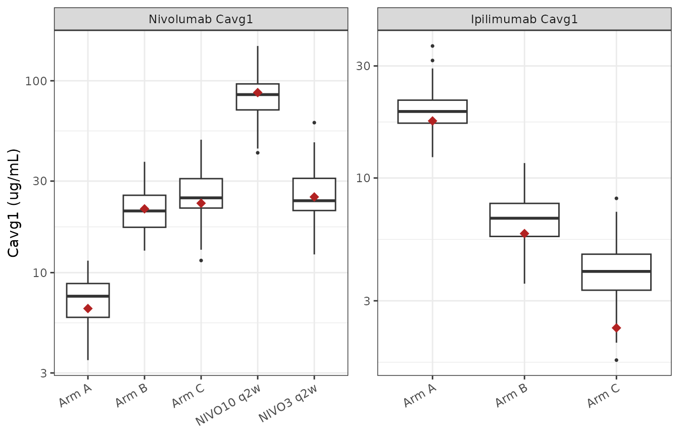
Replicates Figure 1 of Sangro 2023: distribution of first-dose Cavg1 by treatment, regenerated from the published population PK models. Diamonds are the Table S2 geometric means.
Odds and hazard ratios across the regenerated cohort
The regenerated per-patient exposures are passed through both models.
As in Figures 2 and 3, each ratio is taken against nivolumab Cavg1 25
ug/mL without ipilimumab, with all other covariates equal (so only the
two exposure terms contribute). The OS model is solved with
ECOG_GE1 = 0, LDHR = 1 and the Bajaj 2017
reference clearance for every patient, and the same reference patient is
solved at the reference exposure.
er <- cav_nivo |>
  rename(CAV_NIVOLUMAB = cav) |>
  left_join(cav_ipi |> rename(CAV_IPILIMUMAB = cav), by = c("id", "arm")) |>
  mutate(CAV_IPILIMUMAB = dplyr::coalesce(CAV_IPILIMUMAB, 0))

ref_row <- tibble::tibble(id = 0L, arm = "reference", CAV_NIVOLUMAB = cav_ref, CAV_IPILIMUMAB = 0)
er_in <- bind_rows(ref_row, er) |>
  mutate(
    time = 0,
    amt = 0,
    evid = 0L,
    ECOG_GE1 = 0,
    LDHR = 1,
    CLI = 9.4 / 1000,
    sid = dplyr::row_number()
  )
ev_er <- er_in |> select(id = sid, time, amt, evid, CAV_NIVOLUMAB, CAV_IPILIMUMAB, ECOG_GE1, LDHR, CLI)

p_orr <- muffle_no_omega(as.data.frame(rxode2::rxSolve(mod_orr, events = ev_er, returnType = "data.frame")))
p_os <- as.data.frame(rxode2::rxSolve(mod_os, events = ev_er, returnType = "data.frame"))

er_in <- er_in |>
  mutate(
    logit = qlogis(p_orr$prob_orr_central),
    or = exp(logit - logit[1]),
    hr = p_os$hr / p_os$hr[1]
  ) |>
  dplyr::filter(arm != "reference")

fig_bars <- arm_gm |>
  select(arm, or_p05, or_p95, hr_p05, hr_p95)
cohort_ratio <- er_in |>
  group_by(arm) |>
  summarise(
    or_med = median(or),
    or_q05 = quantile(or, 0.05),
    or_q95 = quantile(or, 0.95),
    hr_med = median(hr),
    hr_q05 = quantile(hr, 0.05),
    hr_q95 = quantile(hr, 0.95),
    .groups = "drop"
  ) |>
  left_join(fig_bars, by = "arm")

cohort_ratio |>
  transmute(
    Treatment = arm,
    "OR median (P05-P95)" = sprintf("%.2f (%.2f-%.2f)", or_med, or_q05, or_q95),
    "Figure 2 P05-P95" = ifelse(is.na(or_p05), "--", sprintf("%.2f-%.2f", or_p05, or_p95)),
    "HR median (P05-P95)" = sprintf("%.3f (%.3f-%.3f)", hr_med, hr_q05, hr_q95),
    "Figure 3 P05-P95" = ifelse(is.na(hr_p05), "--", sprintf("%.2f-%.2f", hr_p05, hr_p95))
  ) |>
knitr::kable(caption = "Odds and hazard ratios across the regenerated cohort against the percentile bars of Sangro 2023 Figures 2 and 3.")| Treatment | OR median (P05-P95) | Figure 2 P05-P95 | HR median (P05-P95) | Figure 3 P05-P95 |
|---|---|---|---|---|
| Arm A | 3.46 (3.08-4.04) | 2.92-3.70 | 0.578 (0.538-0.611) | 0.56-0.60 |
| Arm B | 2.09 (1.75-2.38) | 1.05-2.10 | 0.734 (0.698-0.793) | 0.73-0.98 |
| Arm C | 1.66 (1.34-1.95) | 0.83-1.70 | 0.810 (0.756-0.883) | 0.79-1.08 |
| NIVO10 q2w | 0.61 (0.46-0.80) | – | 1.099 (1.059-1.126) | – |
| NIVO3 q2w | 1.01 (0.86-1.07) | 0.95-1.10 | 0.996 (0.971-1.042) | 0.97-1.02 |
# For arms A and B, whose regenerated exposures match Table S2, the cohort
# median ratio must agree with the ratio at the Table S2 geometric means
# (checked against Figures 2 and 3 above). The comparison is on the median,
# not on the published bar edges: arm B's median sits next to the top of its
# Figure 2 bar, and which side of the edge it lands on depends on the random
# draw. Arm C is excluded for the reason given above.
ab <- dplyr::filter(cohort_ratio, arm %in% c("Arm A", "Arm B")) |>
  left_join(select(arm_gm, arm, or_s2, hr_s2), by = "arm")
stopifnot(
  all(abs(ab$or_med / ab$or_s2 - 1) < 0.15),
  all(abs(ab$hr_med / ab$hr_s2 - 1) < 0.15)
)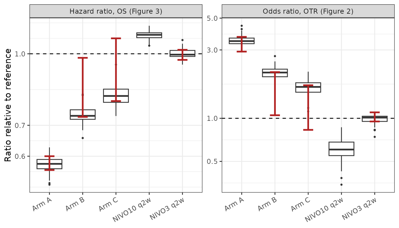
Replicates Figures 2 and 3 of Sangro 2023: per-patient odds ratio of objective response and hazard ratio of death relative to nivolumab Cavg1 25 ug/mL without ipilimumab. Boxes: regenerated cohort; red bars: published P05-P95.
Assumptions and deviations
-
Zero ipilimumab exposure. Both models take the
natural log of ipilimumab Cavg1, which is 0 for every monotherapy
patient. The log term is set to 0 when
CAV_IPILIMUMAB = 0. The paper does not print this choice; it is the only handling that reproduces the arm-level bars of Figures 2 and 3 (see above). - Natural logarithm. “Log-transformed” is read as the natural log for both Cavg1 terms and for LDH/ULN. The Cavg1 base is fixed by Figure 2 (log10 would put arm A’s odds ratio at 1.85, outside 2.92-3.70). The LDH/ULN base cannot be checked against any printed quantity, and the same natural log is assumed.
-
Baseline nivolumab clearance units. Table 3 gives
the coefficient per mL/h. The model takes
CLIin the canonical L/h and multiplies by 1000. -
No baseline hazard. A Cox model leaves h0(t)
unspecified, so the OS model returns the relative hazard
hronly. The predicted Kaplan-Meier curves of Figure S1 cannot be reproduced from the published information. -
Placeholder residual. The logistic model is
deterministic; the fixed additive SD of 0.001 on
prob_orr_centralexists only because rxode2 requires an observation declaration. - Upstream PK. Sangro 2023 used updated refits of the Bajaj 2017 and Sanghavi 2020 models that are not published. This vignette uses the published originals, with assumed infusion durations of 1 hour (nivolumab) and 1.5 hours (ipilimumab), and Table 1-based demographics (log-normal weight around 67 kg, eGFR around 85 mL/min/1.73 m^2 and LDH around 220 U/L, which Table 1 does not report). The regenerated geometric means match Table S2 within 20% for every nivolumab group and for ipilimumab in arms A and B.
- Arm C ipilimumab Cavg1. The regenerated arm C ipilimumab geometric mean is about 70% above Table S2’s 2.3 ug/mL (the Results text gives 1.7). For a single 1 mg/kg dose, the 0-42-day average cannot fall below half the 0-21-day average of arm B unless clearance is materially higher, yet Table S2 gives 2.3 / 5.8 = 0.40 and the text 1.7 / 5.1 = 0.33. The paper does not say how the 6-weekly averaging window was defined, so the discrepancy is reported rather than resolved, and arm C is excluded from the regenerated-cohort gate.
- Two sets of ipilimumab geometric means. The Results text (16.7 / 5.1 / 1.7 ug/mL) and Table S2 (17.5 / 5.8 / 2.3 ug/mL) differ slightly; both are shown above and both satisfy the Figure 2 and 3 checks. Table S2 is used elsewhere because it also gives the nivolumab values.
-
Covariates screened but not retained. OTR:
etiology, PD-L1 status, ECOG, tumor size, extrahepatic spread or
vascular invasion, and baseline nivolumab clearance. OS: etiology,
alpha-fetoprotein, tumor size and albumin. No estimates are reported for
them; they are listed in each model’s
covariatesDataExcluded. - Errata. No erratum or correction to Sangro 2023 was found (checked 2026-11-06).