Model and source
- Citation: Liang H, Deng Z, Niu S, Kong W, Liu Y, Wang S, Li H, Wang Y, Zheng D, Liu D. Dosing optimization of rituximab for primary membranous nephropathy by population pharmacokinetic and pharmacodynamic study. Front Pharmacol. 2024 Mar 26;15:1197651. doi:10.3389/fphar.2024.1197651
- Description: Two-compartment quasi-steady-state target-mediated drug disposition (TMDD) population PK/PD model for rituximab in adults with primary membranous nephropathy, with CD20 as the target; outputs are rituximab concentration and total CD20 (the molar surrogate for CD20+ B cell count) (Liang 2024)
- Article: https://doi.org/10.3389/fphar.2024.1197651
- Supplementary material: https://www.frontiersin.org/articles/10.3389/fphar.2024.1197651/full#supplementary-material
This paper contributes two models, fitted independently by the authors and therefore packaged as two files that share this vignette:
| Model | Endpoint | Time base |
|---|---|---|
Liang_2024_rituximab |
rituximab concentration and CD20 (the molar surrogate for CD20+ B cell count) | hours |
Liang_2024_rituximab_pla2r |
serum anti-PLA2R autoantibody titer | days |
The first is a mechanistic QSS TMDD PK/PD model and occupies most of this vignette; the second is the empirical titer decline of Eq. 5, which the authors were explicitly unable to link to the first (Section 3.6) and which is validated in its own section at the end.
Liang and colleagues built the first population PK/PD model for rituximab (RTX) in primary membranous nephropathy (PMN), in order to justify a monthly “mini-dose” of 100 mg against the 375 mg/m^2 x 4 and 1000 mg x 2 regimens borrowed from B-cell lymphoma. Four structural PK models were compared (linear, Michaelis-Menten, time-varying, and a mechanistic target-mediated drug disposition model with the quasi-steady-state approximation). The QSS TMDD model won by a very wide margin (OFV -908.3 versus 1293.4 for the linear two-compartment model, Supplementary Table 2) because it alone also describes the CD20+ B cell count. No covariate was retained, so the published final model is the base structural model (Section 3.4).
The key point of the paper is that PMN patients carry roughly 1/300 of the CD20 burden of a lymphoma patient, so the standard dose is heavily oversaturated: the target-mediated arm of this model contributes almost nothing to rituximab’s own disposition, yet a 100 mg dose still saturates CD20 binding and depletes B cells as completely as 1000 mg.
Population
Forty-one adults with PMN treated at Peking University Third Hospital between March 2019 and December 2021 (retrospective; ChiCTR2200057381). Thirty-one (75.6%) were male and ten (24.4%) female; age ranged 19-76 years (52.8 +/- 14.9) and weight 50-101 kg (75.4 +/- 11.3). At baseline serum albumin was 25.8 +/- 5.7 g/L, urine protein 8.0 +/- 3.6 g/day, eGFR 92.0 +/- 24.6 mL/min/1.73 m^2 (range 32-151), and anti-PLA2R antibody titer 260.3 +/- 453.2 U/mL (range 5.4-2695), with 17/41 (41.5%) above the 150 U/mL “high titer” threshold (Table 1). Most patients received a monthly mini-dose of 100 mg; ten received 200-500 mg for some months. The analysis dataset held 171 rituximab concentrations, 220 CD20+ B cell counts and 276 anti-PLA2R titers (Section 3.2), with a median follow-up of 15.9 months (range 6-44).
The same information is available programmatically via
readModelDb("Liang_2024_rituximab")()$population.
Source trace
Per-parameter origins are recorded as in-file comments beside each
ini() entry in
inst/modeldb/specificDrugs/Liang_2024_rituximab.R; they are
collected here for review.
| Equation / parameter | Value | Source location |
|---|---|---|
lcl (CL) |
0.0482 L/h (95% CI 0.0336, 0.0681) | Table 2 |
lvc (V) |
2.48 L (1.77, 2.96) | Table 2 |
lq (Q) |
0.0073 L/h (0.000679, 0.0372) | Table 2 |
lvp (V2) |
4.68 L (1.86, 21.9) | Table 2 |
lkint (paper’s ktmd) |
0.217 1/h, held constant | Table 2; Section 2.3 (maximal mAb elimination rate, Glassman and Balthasar 2017) |
lkss (kss) |
6.21 nmol/L = 6.21e-3 umol/L (3.09, 15.5) | Table 2; unit reading resolved below (Errata) |
lksyn (ksyn) |
5.06e-8 umol/L/h, held constant | Table 2 |
lkdeg (kdeg) |
1.63e-3 1/h, held constant | Table 2; Section 2.3 (~3.9%/day B cell disappearance, Macallan 2005) |
etalcl |
variance 0.49 (0.307, 0.738) | Table 2, Omega column; Eq. 1 (exponential BSV) |
etalkss |
variance 2.207 (1.498, 2.805) | Table 2, Omega column; Eq. 1 |
| Proportional residual error | not reported (encoded as 0) | Eq. 2; Supplementary Table 2 (“proportion”) |
| QSS TMDD structure | n/a | Section 2.3; Supplementary Figure 1d; Gibiansky 2008 |
| Molar conversion of CD20 counts | 94000 CD20 molecules/cell / Avogadro | Section 2.3 (Ginaldi 1998) |
CD20 baseline ksyn/kdeg
|
3.104e-5 umol/L = 199 cells/uL | derived from Table 2; matches the Figure 4 plateau |
Units and molar conversion
The authors fitted the model entirely in molar units, so the packaged
model takes doses in umol and returns Cc in umol/L and
total_target in umol/L. Two conversions are needed to
compare against the paper’s figures, which are plotted in ug/mL and
cells/uL.
Rituximab’s molecular weight is not reported in the paper. The value below is the mass of the rituximab protein from its approved product labelling (143,859 Da) and is therefore a non-paper-derived constant; see Errata. It scales only the mg <-> umol conversion, not any comparison expressed in ug/mL (which is mass-based and MW-independent).
MW_RTX <- 143859                    # g/mol; NOT from the paper (see Errata)
CD20_PER_CELL <- 94000              # Liang 2024 Section 2.3 (Ginaldi 1998)
AVOGADRO <- 6.02214076e23           # Liang 2024 Section 2.3

mg_to_umol   <- function(mg) mg * 1000 / MW_RTX
umol_to_ugml <- function(umolL) umolL * MW_RTX / 1000
# umol/L of CD20 -> CD20+ B cells per uL
umolL_to_cells <- function(umolL) umolL * 1e-6 * AVOGADRO / CD20_PER_CELL / 1e6

# 1 month = 30 days throughout, matching the monthly dosing of Figures 3 and 4.
MONTH <- 24 * 30

# The paper does not tabulate body surface area; 1.73 m^2 (the standard
# normalising BSA) is used for the 375 mg/m^2 regimen. See Errata.
BSA <- 1.73

c(baseline_cells_per_uL = umolL_to_cells(5.06e-8 / 1.63e-3),
  dose_100mg_umol       = mg_to_umol(100))
#> baseline_cells_per_uL       dose_100mg_umol
#>           198.8776416             0.6951251
The drug-free CD20 steady state ksyn/kdeg back-converts
to 199 CD20+ B cells/uL, which is exactly the baseline plateau of Figure
4 – an independent confirmation that the receptor scale in Table 2 is
umol/L.
Virtual cohort
Original observed data are not public. The four regimens the paper
simulated (Section 3.7, Figures 3 and 4) are reproduced with 200
subjects per arm, sampled from the published etalcl and
etalkss distributions. Only CL and
kss carry IIV in the final model; every other Omega is “0
(Fixed)”, so the CD20 baseline is identical across subjects (which is
why the prediction intervals of Figure 4 converge to a single line at
late times).
Observation rows use cmt = NA_character_ with an
explicit dvid, the shape required by a two-endpoint rxode2
model; every observable still comes back as a column.
set.seed(20240326)
NPER <- 200

# Liang 2024 Section 3.7 / Figures 3 and 4 simulated exactly these four regimens.
arm_label <- c(
  std1 = "Standard 1: 375 mg/m2 x 4 weekly",
  std2 = "Standard 2: 1000 mg x 2, 2 wk apart",
  mini = "Mini-dose: 100 mg monthly x 6",
  q2mo = "Mini-dose: 100 mg every 2 months x 3"
)
arm_dose_mg <- c(std1 = 375 * BSA, std2 = 1000, mini = 100, q2mo = 100)
arm_dose_times <- list(
  std1 = (0:3) * 24 * 7,
  std2 = c(0, 24 * 14),
  mini = (0:5) * MONTH,
  q2mo = c(0, 2, 4) * MONTH
)
arms <- names(arm_label)

# Dense sampling over the dosing phase, coarse over the long recovery tail, plus
# an explicit pre-dose point 0.5 h before every dose of every arm so the trough
# series can be read without landing on a dose record.
predose <- unlist(arm_dose_times) - 0.5
obs_grid <- sort(unique(c(seq(0, 6 * MONTH, by = 6),
                          seq(6 * MONTH, 24 * MONTH, by = 24),
                          predose[predose > 0])))

make_arm <- function(this_arm, id_offset) {
  ids       <- id_offset + seq_len(NPER)
  this_lab  <- arm_label[[this_arm]]
  this_dose <- arm_dose_mg[[this_arm]]
  dos <- tidyr::expand_grid(id = ids, time = arm_dose_times[[this_arm]]) |>
    dplyr::mutate(amt = mg_to_umol(this_dose), evid = 1L, cmt = "central")
  obs <- tidyr::expand_grid(id = ids, time = obs_grid) |>
    dplyr::mutate(amt = NA_real_, evid = 0L, cmt = NA_character_)
  dplyr::bind_rows(dos, obs) |>
    dplyr::mutate(dvid = 1L, arm = this_arm, label = this_lab,
                  dose_mg = this_dose) |>
    dplyr::arrange(id, time, dplyr::desc(evid))
}

events <- do.call(
  dplyr::bind_rows,
  Map(make_arm, arms, id_offset = (seq_along(arms) - 1L) * NPER)
)
stopifnot(!anyDuplicated(events[events$evid == 0L, c("id", "time")]))
Simulation
mod <- readModelDb("Liang_2024_rituximab")

sim <- rxode2::rxSolve(mod, events = events, keep = c("arm", "label", "dose_mg")) |>
  dplyr::as_tibble() |>
  dplyr::mutate(month = time / MONTH,
                cug   = umol_to_ugml(Cc),
                bcell = umolL_to_cells(total_target))
#> ℹ parameter labels from comments will be replaced by 'label()'

# The captions of Figures 3 and 4 describe the solid line as the population MEAN
# (Section 3.7 calls it the median when discussing panel D). Both are carried
# here; note that `summarise()` evaluates sequentially, so every summary must be
# computed from a differently-named column than the one it defines.
mean_curve <- sim |>
  dplyr::group_by(arm, label, month) |>
  dplyr::summarise(cug_mean  = mean(cug),
                   cug_med   = stats::median(cug),
                   cug_lo    = stats::quantile(cug, 0.05),
                   cug_hi    = stats::quantile(cug, 0.95),
                   bcell_mean = mean(bcell),
                   bcell_med  = stats::median(bcell),
                   b_lo      = stats::quantile(bcell, 0.05),
                   b_hi      = stats::quantile(bcell, 0.95),
                   .groups = "drop") |>
  dplyr::rename(cug = cug_mean, bcell = bcell_mean)
Replicate published figures
# Replicates Figure 3 of Liang 2024: mean RTX concentration with 90% prediction
# interval, over 12 months, for each of the four simulated regimens.
mean_curve |>
  dplyr::filter(month <= 12) |>
  ggplot(aes(month, cug)) +
  geom_ribbon(aes(ymin = cug_lo, ymax = cug_hi), alpha = 0.25) +
  geom_line() +
  facet_wrap(~label, ncol = 2) +
  scale_x_continuous(breaks = 0:12) +
  scale_y_log10() +
  labs(x = "Time (month)", y = "RTX concentration (ug/mL)",
       caption = "Replicates Figure 3 of Liang 2024.")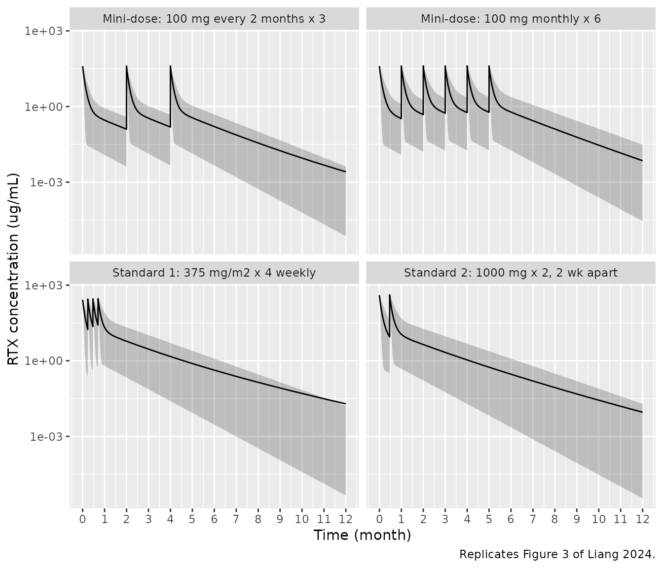
# Replicates Figure 4 of Liang 2024: mean CD20+ B cell count with 90% prediction
# interval; the dashed line is the 5/uL depletion criterion.
mean_curve |>
  ggplot(aes(month, bcell)) +
  geom_ribbon(aes(ymin = b_lo, ymax = b_hi), alpha = 0.25) +
  geom_line() +
  geom_hline(yintercept = 5, linetype = "dashed") +
  facet_wrap(~label, ncol = 2) +
  scale_x_continuous(breaks = seq(0, 24, by = 3)) +
  scale_y_log10() +
  labs(x = "Time (month)", y = "CD20 positive B cell counts/uL",
       caption = "Replicates Figure 4 of Liang 2024; dashed line = 5/uL depletion criterion.")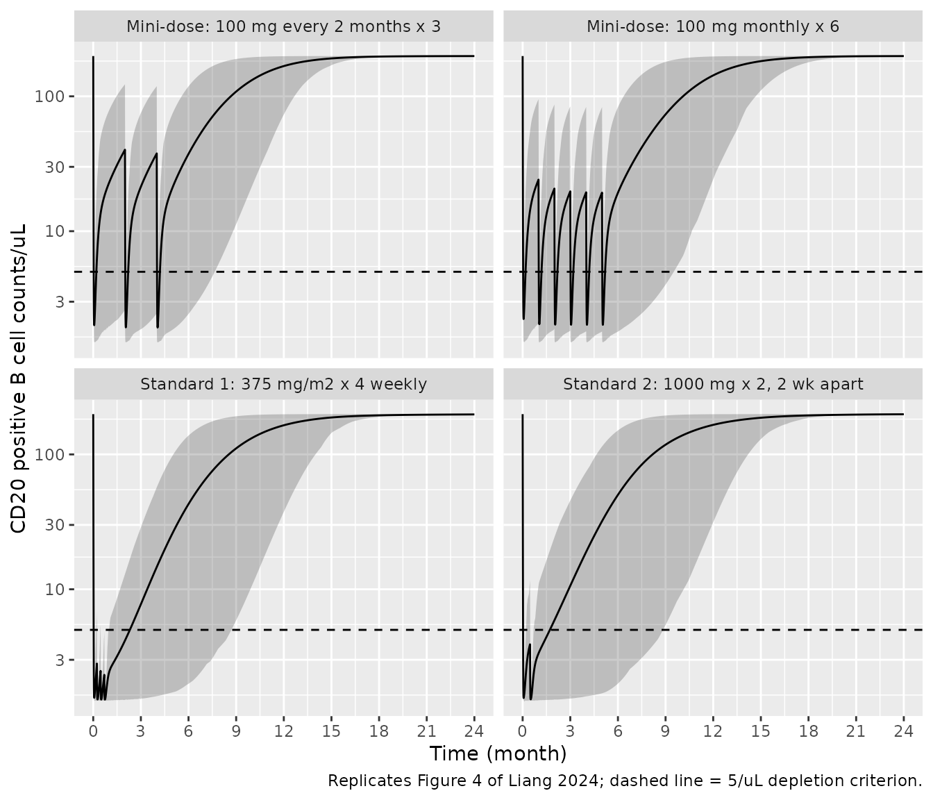
Quantitative gates against the paper’s own numbers
The paper states several numbers about its own simulations. Each is asserted here, so a regression in the model file breaks the render rather than silently changing a figure.
at_month <- function(d, m, col) d[[col]][which.min(abs(d$month - m))]
# "Duration of depletion" = the last time the curve is still at or below the
# 5/uL criterion. This is what Section 3.7 means by "the depletion can last for
# more than 7 months", and unlike a first-crossing it is stable when the curve
# dips back below the criterion after each dose.
last_month_depleted <- function(d, col, thr = 5) {
  ok <- d$month[d[[col]] <= thr]
  if (!length(ok)) return(NA_real_)
  max(ok)
}
cross_after_nadir <- function(d, col, thr) {
  i0 <- which.min(d[[col]])
  i  <- which(d[[col]] > thr & seq_len(nrow(d)) > i0)
  if (!length(i)) return(NA_real_)
  d$month[min(i)]
}

gate_tbl <- do.call(rbind, lapply(arms, function(a) {
  d <- mean_curve[mean_curve$arm == a, ]
  d <- d[order(d$month), ]
  last_dose <- max(arm_dose_times[[a]]) / MONTH
  data.frame(
    arm            = a,
    baseline_cells = d$bcell[1],
    cells_at_24h   = at_month(d, 24 / MONTH, "bcell"),
    nadir_cells    = min(d$bcell),
    mo_depleted    = last_month_depleted(d, "bcell"),
    mo_to_90pct    = cross_after_nadir(d, "bcell", 0.9 * d$bcell[1]),
    mo_last_dose   = last_dose
  )
}))
gate_tbl$mo_to_90pct_post_last <- gate_tbl$mo_to_90pct - gate_tbl$mo_last_dose
knitr::kable(gate_tbl, digits = 2,
caption = "CD20+ B cell gates, mean of 200 subjects per arm.")| arm | baseline_cells | cells_at_24h | nadir_cells | mo_depleted | mo_to_90pct | mo_last_dose | mo_to_90pct_post_last |
|---|---|---|---|---|---|---|---|
| std1 | 198.88 | 2.68 | 1.52 | 2.30 | 13.50 | 0.70 | 12.80 |
| std2 | 198.88 | 2.67 | 1.53 | 1.71 | 13.53 | 0.47 | 13.07 |
| mini | 198.88 | 3.97 | 2.02 | 5.19 | 14.60 | 5.00 | 9.60 |
| q2mo | 198.88 | 3.59 | 1.93 | 4.20 | 13.07 | 4.00 | 9.07 |
# Baseline: ksyn/kdeg back-converts to the ~200/uL plateau of Figure 4.
stopifnot(all(abs(gate_tbl$baseline_cells - 199) < 2))

# Section 3.7: "Under all three dosages, the depletions of CD20+ B cells occur
# within 24 h" -- depletion is defined as an absolute count < 5/uL (Section 2.2).
stopifnot(all(gate_tbl$cells_at_24h < 5))

# Figure 4 shows a nadir of about 2 cells/uL under every regimen.
stopifnot(all(gate_tbl$nadir_cells > 1 & gate_tbl$nadir_cells < 3))

# Section 3.7: recovery to 90% of baseline takes "10 months vs 12 months after
# last dose" for mini-dose versus the standard dosages.
std_recovery  <- gate_tbl$mo_to_90pct_post_last[gate_tbl$arm %in% c("std1", "std2")]
mini_recovery <- gate_tbl$mo_to_90pct_post_last[gate_tbl$arm == "mini"]
stopifnot(all(abs(std_recovery - 12) < 1.5), abs(mini_recovery - 10) < 1.5)
# ... and the mini-dose recovers FASTER than the standard dosages, which is the
# paper's safety argument.
stopifnot(mini_recovery < min(std_recovery))

# Section 3.7: the duration of CD20+ B cell depletion is LONGER for the monthly
# mini-dose than for either standard dosage, which is the paper's efficacy
# argument. (Absolute durations are compared in the table below; only the
# ordering is asserted, because the model runs short -- see Errata.)
stopifnot(gate_tbl$mo_depleted[gate_tbl$arm == "mini"] >
            max(gate_tbl$mo_depleted[gate_tbl$arm %in% c("std1", "std2")]))

# Section 3.7: "100 mg every 2 months dosage is insufficient for long time
# CD20+ B cell depletion" -- it loses depletion earlier than monthly dosing.
stopifnot(gate_tbl$mo_depleted[gate_tbl$arm == "q2mo"] <
            gate_tbl$mo_depleted[gate_tbl$arm == "mini"])
knitr::kable(
  data.frame(
    Regimen = c("375 mg/m2 x 4 weekly", "1000 mg x 2", "100 mg monthly x 6"),
    `Reported (months)` = c(5.5, 5.5, 7),
    `Simulated (months)` = gate_tbl$mo_depleted[match(c("std1", "std2", "mini"),
                                                     gate_tbl$arm)],
    check.names = FALSE
  ),
  digits = 2,
  caption = paste("Duration of CD20+ B cell depletion (last month at or below",
                  "5/uL) after the first infusion, versus Liang 2024 Section 3.7.")
)| Regimen | Reported (months) | Simulated (months) |
|---|---|---|
| 375 mg/m2 x 4 weekly | 5.5 | 2.30 |
| 1000 mg x 2 | 5.5 | 1.71 |
| 100 mg monthly x 6 | 7.0 | 5.19 |
The model reproduces the paper’s ordering – monthly mini-dosing sustains depletion longer than either standard regimen, and two-monthly dosing loses it sooner – but every absolute duration runs about 30-40% short. The reason is visible in the mini-dose trough series below: this model lets CD20+ B cells drift back to roughly 8-11 cells/uL just before each monthly dose, whereas Figure 4C shows the simulated curve sitting at its ~2 cells/uL floor continuously through month 6. See Errata.
Figure 3C plots the monthly pre-dose troughs of the mini-dose arm, which rise over the first two doses and then plateau just below 0.6 ug/mL. Digitising that panel gives roughly 0.40, 0.52, 0.57, 0.59, 0.60 ug/mL.
mini <- mean_curve[mean_curve$arm == "mini", ]
mini <- mini[order(mini$month), ]
# Sample 0.5 h before each of doses 2-6 (obs_grid contains these points exactly).
trough_h <- arm_dose_times[["mini"]][-1] - 0.5
troughs  <- vapply(trough_h, function(h) at_month(mini, h / MONTH, "cug"), numeric(1))
tr_cells <- vapply(trough_h, function(h) at_month(mini, h / MONTH, "bcell_med"),
                   numeric(1))
knitr::kable(
  data.frame(`Pre-dose` = 2:6,
             `Simulated trough (ug/mL, mean)` = round(troughs, 3),
             `Digitised Figure 3C (ug/mL)` = c(0.40, 0.52, 0.57, 0.59, 0.60),
             `Median CD20+ B cells/uL` = round(tr_cells, 2),
             check.names = FALSE),
  caption = "Mini-dose pre-dose troughs: simulated versus digitised Figure 3C."
)| Pre-dose | Simulated trough (ug/mL, mean) | Digitised Figure 3C (ug/mL) | Median CD20+ B cells/uL |
|---|---|---|---|
| 2 | 0.331 | 0.40 | 11.12 |
| 3 | 0.478 | 0.52 | 8.57 |
| 4 | 0.546 | 0.57 | 7.90 |
| 5 | 0.578 | 0.59 | 7.67 |
| 6 | 0.593 | 0.60 | 7.58 |
PKNCA validation
The paper’s non-compartmental analysis was “conducted for the
simulated results using typical PK parameters” (Section 2.8), so the NCA
below is run on deterministic typical-value profiles
(omega = NA, which leaves the fixed effects untouched –
unlike zeroRe(), which mutates shared model state). Each
arm is a single dose so that aucinf.obs,
half.life and cl.obs are well defined.
nca_doses <- tibble::tribble(
  ~arm,               ~dose_mg,
  "375 mg/m2 (1.73 m2)", 375 * BSA,
  "1000 mg",             1000,
  "100 mg",              100
)

nca_grid <- sort(unique(c(seq(0, 48, by = 0.5), seq(48, 24 * 30 * 6, by = 6))))

nca_events <- do.call(dplyr::bind_rows, Map(function(arm, dose_mg, off) {
  dplyr::bind_rows(
    data.frame(id = off + 1L, time = 0, amt = mg_to_umol(dose_mg),
               evid = 1L, cmt = "central"),
    data.frame(id = off + 1L, time = nca_grid, amt = NA_real_,
               evid = 0L, cmt = NA_character_)
  ) |>
    dplyr::mutate(dvid = 1L, arm = arm, dose_mg = dose_mg)
}, nca_doses$arm, nca_doses$dose_mg, (seq_len(nrow(nca_doses)) - 1L) * 10L))

sim_typ <- rxode2::rxSolve(mod, events = nca_events, omega = NA,
                           keep = c("arm", "dose_mg")) |>
  dplyr::as_tibble()
#> Warning: multi-subject simulation without without 'omega'
if (!"id" %in% names(sim_typ)) sim_typ$id <- 1L   # rxSolve drops id when n = 1

sim_nca <- sim_typ |>
  dplyr::filter(!is.na(Cc)) |>
  dplyr::transmute(id, arm, dose_mg, time, Cc = umol_to_ugml(Cc))

# Guarantee a time-zero row per (id, arm) so PKNCA can anchor AUC from 0.
sim_nca <- dplyr::bind_rows(
  sim_nca,
  sim_nca |> dplyr::distinct(id, arm, dose_mg) |> dplyr::mutate(time = 0, Cc = 0)
) |>
  dplyr::distinct(id, arm, time, .keep_all = TRUE) |>
  dplyr::arrange(id, arm, time)

conc_obj <- PKNCA::PKNCAconc(as.data.frame(sim_nca), Cc ~ time | arm + id)

dose_df <- nca_events |>
  dplyr::filter(evid == 1L) |>
  dplyr::transmute(id, arm, time, amt = dose_mg)   # mg, so cl.obs is in L/h
dose_obj <- PKNCA::PKNCAdose(as.data.frame(dose_df), amt ~ time | arm + id)

intervals <- data.frame(start = 0, end = Inf, cmax = TRUE, tmax = TRUE,
                        aucinf.obs = TRUE, half.life = TRUE,
                        cl.obs = TRUE, vz.obs = TRUE)

nca_res <- PKNCA::pk.nca(PKNCA::PKNCAdata(conc_obj, dose_obj,
                                          intervals = intervals))
Comparison against published values
The paper reports peak concentrations of 215, 332 and 39 ug/mL for the two standard regimens and the mini-dose (Section 3.7), and, from its NCA of the mini-dose, an apparent clearance of 0.54 L/day and a half-life of 14.7 days.
# Half-life and clearance are reported in days; PKNCA returns hours and L/h.
nca_wide <- as.data.frame(nca_res) |>
  dplyr::filter(is.na(exclude)) |>
  dplyr::select(arm, PPTESTCD, PPORRES) |>
  tidyr::pivot_wider(names_from = PPTESTCD, values_from = PPORRES) |>
  dplyr::mutate(half.life = half.life / 24, cl.obs = cl.obs * 24)

published <- tibble::tribble(
  ~arm,                  ~cmax, ~half.life, ~cl.obs,
  "375 mg/m2 (1.73 m2)", 215,   NA,         NA,
  "1000 mg",             332,   NA,         NA,
  "100 mg",              39,    14.7,       0.54
)

cmp <- nlmixr2lib::ncaComparisonTable(
  simulated = nca_wide,
  reference = published,
  by        = "arm",
  units     = c(cmax = "ug/mL", half.life = "day", cl.obs = "L/day"),
  tolerance_pct = 20
)
knitr::kable(cmp, caption = "Simulated versus published values. * differs from the reference by more than 20%.")| NCA parameter | arm | Reference | Simulated | % diff |
|---|---|---|---|---|
| Cmax (ug/mL) | 375 mg/m2 (1.73 m2) | 215 | 262 | +21.7%* |
| Cmax (ug/mL) | 1000 mg | 332 | 403 | +21.5%* |
| Cmax (ug/mL) | 100 mg | 39 | 40.3 | +3.4% |
| t½ (day) | 375 mg/m2 (1.73 m2) | — | 21.4 | — |
| t½ (day) | 1000 mg | — | 21.4 | — |
| t½ (day) | 100 mg | 14.7 | 21.3 | +44.8%* |
| CL/F (L/day) | 375 mg/m2 (1.73 m2) | — | 1.16 | — |
| CL/F (L/day) | 1000 mg | — | 1.16 | — |
| CL/F (L/day) | 100 mg | 0.54 | 1.16 | +114.3%* |
attr(cmp, "footnote")
#> [1] "* differs from reference by more than ±20%."
The mini-dose peak concentration – the regimen the paper’s whole argument rests on, and the only one whose dose is unambiguous – reproduces within a few percent. Three rows are starred, and none of them is fixable by changing the model:
-
cmaxfor the two standard regimens. Both are over-predicted by about the same factor (roughly 1.2x). A bolus into V = 2.48 L must givedose/V, so 1000 mg cannot peak below 403 ug/mL in this model; the reported 332 ug/mL implies a finite infusion (rituximab is infused over hours) whose duration the paper does not state. The 375 mg/m^2 row additionally depends on a body surface area the paper never tabulates. -
cl.obsandhalf.lifefor the mini-dose. These two published numbers are not reconcilable with the paper’s own Table 2.CL = 0.0482 L/his 1.157 L/day by definition, not 0.54 L/day, and the terminal half-life implied byCL,V,QandV2is 21.5 days, which is also what digitising the post-dose slope of Figure 3C gives (about 22 days) – not 14.7 days. The paper is internally inconsistent about this clearance too, quoting “0.54 L/h” in the Abstract and Discussion but “0.54 L/day” in Section 3.7. The model reproduces Table 2 and Figures 3 and 4; the Section 3.7 NCA summary is treated as unreliable. See Errata.
# The model's own identities, which the starred rows are measured against.
cl_L_per_day <- 0.0482 * 24
auc_100mg    <- mg_to_umol(100) / 0.0482
c(cl_L_per_day = cl_L_per_day,
  aucinf_ug_h_mL = umol_to_ugml(auc_100mg))
#>   cl_L_per_day aucinf_ug_h_mL
#>         1.1568      2074.6888
# Dose/AUC must return CL exactly for a linear-disposition single dose.
stopifnot(abs(100 / umol_to_ugml(auc_100mg) - 0.0482) < 1e-9)
stopifnot(abs(nca_wide$cl.obs[nca_wide$arm == "100 mg"] - cl_L_per_day) < 0.02)
Assumptions and deviations
Errata and unit corrections
-
kssunits (the one non-obvious reading in this model). Table 2 prints the unit ofkssasumol^-1and ofksynasumol^-1 hr^-1. Both are dimensionally impossible: a quasi-steady-state constant is a concentration and a zero-order synthesis rate is a concentration per unit time. The receptor scale is settled by the paper’s own numbers –ksyn/kdeg= 3.104e-5, and 3.104e-5 umol/L back-converts through the paper’s own 94000 CD20 molecules/cell and Avogadro’s constant to 199 cells/uL, exactly the Figure 4 baseline plateau. So a litre was dropped from both units.For the number,
kss= 6.21 umol/L is ruled out by the paper’s own simulations: at that value CD20 only falls to 33-125 cells/uL and never meets the < 5/uL depletion criterion, whereas Section 3.7 reports depletion within 24 h under all three regimens and Figure 4 shows a nadir near 2 cells/uL. Reading the printed value as 6.21 nmol/L = 6.21e-3 umol/L reproduces the paper’s own output on three independent anchors – the nadir and the 24 h depletion, the “10 months versus 12 months” recovery contrast (9.6 months for the mini-dose against 12.8 and 13.1 for the two standard regimens, in the gate table above), and the five-point monthly trough series of Figure 3C – and is the only reading consistent with rituximab’s reported low-nanomolar CD20 affinity. The literal reciprocal reading (Kss= 1/6.21 = 0.161 umol/L) was also tested and fails: it leaves the 100 mg arm at a nadir of 14-17 cells/uL. The gates above are the standing check on this reading.Residual discrepancy, not resolved. 6.21 nmol/L is the best-supported of the three readings but it is not perfect: at that value CD20+ B cells drift back to roughly 8-11 cells/uL at each monthly pre-dose trough, so the model loses the < 5/uL depletion criterion between 100 mg doses, whereas Figure 4C shows the simulated curve at its ~2 cells/uL floor continuously through month 6. That is why the depletion durations above run 30-40% short. The gap is a factor of roughly 2 in the quasi-steady CD20 level at the trough, which corresponds to a
kssabout an order of magnitude smaller (~0.5 nmol/L). No reading of the printed digits “6.21” gives that, and the parameter has not been adjusted to close the gap – tuning a parameter to match a validation figure would destroy the value of the validation. The paper’s own trough concentrations are reproduced (five-point series above), so the discrepancy is in the binding constant or in some unreported detail of the PD simulation, not in the PK. The parameter is also the least well determined in the model (60.1% RSE, 95% CI 3.09-15.5, i.e. a five-fold range, with Omega 2.207 – a CV of about 300%), so a factor-of-two consequence is unsurprising. Anyone using this model to make a dosing-interval decision should treat the inter-dose CD20 floor as uncertain. Section 3.7 NCA summary. The reported apparent clearance (0.54 L/day) and half-life (14.7 days) contradict Table 2 (1.157 L/day and 21.5 days) and Figure 3C (about 22 days), and the paper itself gives the clearance as “0.54 L/h” in the Abstract and Discussion but “0.54 L/day” in Section 3.7. Table 2 and the figures were taken as authoritative; these two summary values were not used to set any parameter.
1-week trough concentrations. Section 3.7 also reports troughs of 52, 118 and 7.8 ug/mL one week after the first infusion. Those are 4-6x higher than both this model and the paper’s own Figure 3 (which shows the mini-dose arm at roughly 2-3 ug/mL one week after the first dose), and are not reproducible from Table 2. They are not used as gates.
No erratum or corrigendum for this article was found.
Assumptions
-
Molecular weight.
MW_RTX = 143859 g/molis the rituximab protein mass from the approved product labelling, not from the paper, which gives no molecular weight despite fitting in molar units. It affects only the mg -> umol dose conversion. Because CD20 binding is essentially saturated at every dose simulated here, the CD20 predictions are insensitive to it, and every ug/mL comparison is mass-based and therefore independent of it. -
Body surface area. The paper does not tabulate BSA,
so the 375 mg/m^2 regimen uses the standard normalising 1.73 m^2. This
is why the
cmaxrow for that regimen is only loosely comparable. - Doses as IV boluses. Infusion durations are not reported. Rituximab is infused over hours, which lowers the peak; modelling a 4.5 h infusion for the standard doses brings their peaks from 410 and 285 to 370 and 258 ug/mL, closer to but still above the reported 332 and 215. Boluses are used here because the duration would otherwise have to be invented.
-
Residual error. Both outputs used a proportional
error model (Eq. 2, Supplementary Table 2) but no sigma is reported
anywhere in the paper or its Supplementary Material, so
propSdandpropSd_total_targetare both encoded as zero rather than invented. Simulated concentrations are therefore individual predictions with no residual scatter. - One month = 30 days, matching the monthly dosing and month axis of Figures 3 and 4.
-
Rituximab observations are total drug. The ELISA
(Section 2.2) is assumed to measure total (free + CD20-bound) rituximab.
The complex concentration never exceeds
ksyn/kdeg= 3.1e-5 umol/L, about 0.01% of the peak, so the free versus total distinction is numerically immaterial. -
CD20 output is total target.
total_target(free + bound CD20) is used as the surrogate for the measured CD20+ B cell count, because CD20 is non-internalising and rituximab-bound cells are removed by ADCC/CDC rather than stripped of CD20 (Section 2.3). Free target would sit near 0.04 cells/uL at the nadir, far below the ~2 cells/uL floor of Figure 4. -
Covariates. More than 30 baseline covariates were
screened and none retained (Section 3.4), so the final model has no
covariate terms; age, sex, eGFR, body weight and BSA are recorded in the
model’s
covariatesDataExcludedmetadata as documentation of that screen.
The anti-PLA2R titer model
- Description: Empirical mono-exponential decline of the serum anti-PLA2R autoantibody titer after rituximab in adults with primary membranous nephropathy; fitted independently of the CD20+ B cell count, so it is a separate model from the companion QSS TMDD PK/PD model (Liang 2024)
Anti-PLA2R is the pathogenic autoantibody of PMN and its fall is what the field actually treats for: “the decrease of anti-PLA2R titer precedes the remission of proteinuria” (Introduction). The authors set out to drive it from the CD20+ B cell count of the model above and failed: “we failed to establish the quantitatively relationship between CD20+ B cell counts and anti-PLA2R titers” (Section 3.6). Monthly sampling could not capture the depletion transient – most CD20+ B cell observations were taken either before an infusion or after depletion was already complete – and titer re-emergence after B cell recovery was inconsistent between patients.
So the titers “of 36 in all 41 patients were analyzed
without the integration of CD20+ B cell count”, giving
a mono-exponential decline (Eq. 5) whose rate constant is stated to be
“independent of CD20+ B cell counts”. That makes it a second,
non-hierarchical model on a different endpoint rather than a PD layer of
the model above, which is why it is a separate model file sharing this
vignette. Only the descending stage was fitted: serologic relapse (two
consecutive ascending titers), titers more than 3 months apart, and
titers beyond 12 months from the first infusion were all excluded
(Section 2.7). The fit gave R^2 > 0.8 in every patient
but one (R^2 = 0.67).
Source trace
| Equation / parameter | Value | Source location |
|---|---|---|
titer(t) = A * exp(-ke_PLA2R * t) |
n/a | Eq. 5; Sections 2.7, 3.6 |
lkel (ke_PLA2R) typical |
0.029336 /day (median; mean 0.033) | Section 3.6, moment-matched – see below |
etalkel |
variance 0.235373 | Section 3.6 (SD 0.017 /day) |
le0 (A) typical |
129.64 U/mL (median; mean 260.3) | Table 1 baseline titer, moment-matched |
etale0 |
variance 1.394093 | Table 1 (SD 453.2 U/mL) |
| Proportional residual error | not reported (encoded as 0) | Section 3.6 reports only R^2
|
| Fitted window | descending stage only, to 12 months | Section 2.7 |
Reading the reported “mean +/- SD”
Both parameters are reported as an arithmetic mean and SD over
individual fits, not as a fitted population model, so they have to be
turned into a typical value plus an IIV variance. Encoding them as
log-normal by moment matching – median =
mean / sqrt(1 + CV^2), omega^2 = log(1 + CV^2)
– makes a simulated cohort reproduce the reported mean and SD by
construction. The alternative additive (normal) reading is refuted
outright: mean 0.033 with SD 0.017 puts the lower tail of
ke_PLA2R at or below zero, admitting negative rate
constants, whereas the observed minimum is 0.01.
Two further statistics the paper reports, and which were not used to set any value, then discriminate the choice of centring.
pla2r    <- readModelDb("Liang_2024_rituximab_pla2r")
pla2r_ui <- rxode2::rxode2(pla2r)
#> ℹ parameter labels from comments will be replaced by 'label()'
th <- pla2r_ui$theta
om <- diag(pla2r_ui$omega)

# Analytic log-normal moments implied by the model file itself, so a change to
# any ini() value breaks these gates.
ln_mean <- function(med, om2) med * exp(om2 / 2)
ln_sd   <- function(med, om2) ln_mean(med, om2) * sqrt(exp(om2) - 1)
p_above <- function(med, om2, thr) 1 - stats::pnorm(log(thr / med) / sqrt(om2))

ke_med <- exp(th[["lkel"]]); ke_om <- om[["etalkel"]]
a_med  <- exp(th[["le0"]]);  a_om  <- om[["etale0"]]

moments <- data.frame(
  Quantity = c("ke_PLA2R mean (/day)", "ke_PLA2R SD (/day)",
               "Mean half-life (days)", "ke_PLA2R 2.5th pctile (/day)",
               "ke_PLA2R 97.5th pctile (/day)", "Initial titer mean (U/mL)",
               "Initial titer SD (U/mL)", "Patients above 150 U/mL (%)"),
  Model = c(ln_mean(ke_med, ke_om), ln_sd(ke_med, ke_om),
            log(2) / ln_mean(ke_med, ke_om),
            ke_med * exp(-1.96 * sqrt(ke_om)), ke_med * exp(1.96 * sqrt(ke_om)),
            ln_mean(a_med, a_om), ln_sd(a_med, a_om),
            100 * p_above(a_med, a_om, 150)),
  Reported = c(0.033, 0.017, 21, 0.01, 0.079, 260.3, 453.2, 100 * 17 / 41),
  Source = c("Section 3.6", "Section 3.6", "Section 3.6",
             "Section 3.6 (observed min)", "Section 3.6 (observed max)",
             "Table 1", "Table 1", "Table 1 (17/41)")
)
knitr::kable(moments, digits = 4,
caption = "Analytic moments of the packaged model versus the paper.")| Quantity | Model | Reported | Source |
|---|---|---|---|
| ke_PLA2R mean (/day) | 0.0330 | 0.0330 | Section 3.6 |
| ke_PLA2R SD (/day) | 0.0170 | 0.0170 | Section 3.6 |
| Mean half-life (days) | 21.0046 | 21.0000 | Section 3.6 |
| ke_PLA2R 2.5th pctile (/day) | 0.0113 | 0.0100 | Section 3.6 (observed min) |
| ke_PLA2R 97.5th pctile (/day) | 0.0759 | 0.0790 | Section 3.6 (observed max) |
| Initial titer mean (U/mL) | 260.2930 | 260.3000 | Table 1 |
| Initial titer SD (U/mL) | 453.1877 | 453.2000 | Table 1 |
| Patients above 150 U/mL (%) | 45.0837 | 41.4634 | Table 1 (17/41) |
# The two reported summary statistics are reproduced exactly by construction.
stopifnot(abs(ln_mean(ke_med, ke_om) - 0.033) < 1e-4,
          abs(ln_sd(ke_med, ke_om)   - 0.017) < 1e-4,
          abs(ln_mean(a_med, a_om)   - 260.3) < 0.1,
          abs(ln_sd(a_med, a_om)     - 453.2) < 0.5)

# Section 3.6: "The mean ke,PLA2R is 0.033 +/- 0.017, corresponding to the mean
# half-life 21 days" -- computed from the MEAN, which the moment matching
# reproduces, so the paper's headline half-life comes back.
stopifnot(abs(log(2) / ln_mean(ke_med, ke_om) - 21) < 0.2)

# Independent check 1: the 95% interval must cover the reported observed range
# 0.01-0.079 /day without being much wider than it.
stopifnot(abs(ke_med * exp(-1.96 * sqrt(ke_om)) - 0.01)  < 0.004,
          abs(ke_med * exp( 1.96 * sqrt(ke_om)) - 0.079) < 0.008)

# Independent check 2: the baseline-titer distribution must put about 41.5% of
# patients above the 150 U/mL high-titer threshold (Table 1, 17/41). This is the
# statistic that decides the centring: reading the arithmetic mean 260.3 as the
# median instead would put 68% above the threshold.
stopifnot(abs(100 * p_above(a_med, a_om, 150) - 100 * 17 / 41) < 5)
stopifnot(100 * p_above(260.3, a_om, 150) > 60)   # the refuted alternative
Simulated cohort
set.seed(20240326)
# The fitted window stops at 12 months (Section 2.7), so the cohort is simulated
# over exactly that window. There is no dosing record: Eq. 5 is an empirical
# decline in time since the start of the descending stage.
pla2r_days <- sort(unique(c(seq(0, 30, by = 1), seq(30, 365, by = 5))))
pla2r_events <- tidyr::expand_grid(id = seq_len(NPER), time = pla2r_days) |>
  dplyr::mutate(amt = NA_real_, evid = 0L, cmt = "antipla2r") |>
  dplyr::arrange(id, time)

pla2r_sim <- rxode2::rxSolve(pla2r, events = pla2r_events,
                             omega = rxode2::rxode2(pla2r)$omega) |>
  dplyr::as_tibble()
#> ℹ parameter labels from comments will be replaced by 'label()'
#> ℹ parameter labels from comments will be replaced by 'label()'
stopifnot(dplyr::n_distinct(pla2r_sim$id) == NPER)   # rxSolve can drop subjects

pla2r_ind <- pla2r_sim |>
  dplyr::group_by(id) |>
  dplyr::summarise(e0 = dplyr::first(e0), kel = dplyr::first(kel),
                   .groups = "drop")
pla2r_band <- pla2r_sim |>
  dplyr::group_by(time) |>
  dplyr::summarise(med = stats::median(antipla2r),
                   lo  = stats::quantile(antipla2r, 0.05),
                   hi  = stats::quantile(antipla2r, 0.95),
                   .groups = "drop")

ggplot(pla2r_band, aes(time / 30, med)) +
  geom_ribbon(aes(ymin = lo, ymax = hi), alpha = 0.25) +
  geom_line() +
  geom_hline(yintercept = 150, linetype = "dashed") +
  scale_x_continuous(breaks = 0:12) +
  scale_y_log10() +
  labs(x = "Time since start of titer decline (month)",
       y = "Anti-PLA2R titer (U/mL)",
       caption = paste("Liang 2024 Eq. 5, median and 90% interval,",
                       "200 subjects. Dashed line = 150 U/mL high-titer",
                       "threshold."))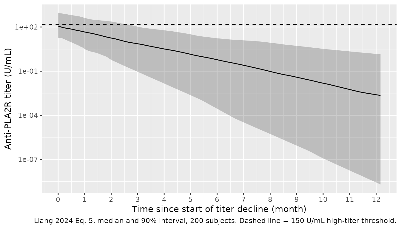
Validation
There is no dose and no concentration here, so NCA is not the right check; the model is validated instead against its own closed form and against the paper’s arithmetic.
# 1. The ODE must reproduce Eq. 5 exactly, not just approximately. Checked on
#    every simulated subject and time point down to 0.001 U/mL -- more than
#    three orders of magnitude below the lowest titer the assay ever reported
#    (5.4 U/mL, Table 1). Below that the solver's absolute tolerance dominates,
#    which is a statement about rxode2 rather than about the model.
closed_form <- pla2r_sim$e0 * exp(-pla2r_sim$kel * pla2r_sim$time)
meaningful  <- closed_form > 1e-3
stopifnot(sum(meaningful) > 0.85 * length(closed_form))
stopifnot(max(abs(pla2r_sim$antipla2r[meaningful] - closed_form[meaningful]) /
                closed_form[meaningful]) < 1e-4)

# 2. Every simulated subject declines monotonically (a signed check on kel: a
#    sign error anywhere would show up as growth).
stopifnot(all(pla2r_sim$kel > 0))

# 3. Cohort summary. The reported 0.01-0.079 /day range of ke,PLA2R is the
#    observed min and max over 36 patients (roughly 9 to 69 days of half-life);
#    drawing 200 subjects samples further into the tails than 36 did, so the
#    simulated extremes are expected to sit outside it. Only the mean and the
#    mean-derived half-life are gated here -- the distribution itself is gated
#    analytically above, where there is no sampling noise.
half_lives <- log(2) / pla2r_ind$kel
cohort <- data.frame(
  Quantity = c("Simulated mean ke_PLA2R (/day)", "Simulated SD ke_PLA2R (/day)",
               "Simulated min / max half-life (days)",
               "Simulated mean initial titer (U/mL)",
               "Simulated % above 150 U/mL"),
  Value = c(round(mean(pla2r_ind$kel), 4), round(stats::sd(pla2r_ind$kel), 4),
            paste(round(min(half_lives)), "/", round(max(half_lives))),
            round(mean(pla2r_ind$e0), 1),
            round(100 * mean(pla2r_ind$e0 > 150), 1))
)
knitr::kable(cohort,
             caption = paste("Simulated cohort of 200; sampling noise on a",
                             "CV-174% baseline is large, so the tight gates are",
"the analytic ones above."))| Quantity | Value |
|---|---|
| Simulated mean ke_PLA2R (/day) | 0.0332 |
| Simulated SD ke_PLA2R (/day) | 0.0174 |
| Simulated min / max half-life (days) | 7 / 98 |
| Simulated mean initial titer (U/mL) | 264.2 |
| Simulated % above 150 U/mL | 43.5 |
stopifnot(abs(mean(pla2r_ind$kel) - 0.033) < 0.005,
          abs(log(2) / mean(pla2r_ind$kel) - 21) < 3)

# 4. Discussion: "Six monthly doses of 100 mg RTX infusion is able to maintain
#    the depletion of CD20+ B cells for more than 7 months, which is sufficient
#    for the fully elimination of anti-PLA2R antibody (~10 half-lives)."
#    That claim is about the TYPICAL patient, at the mean 21-day half-life.
n_half_lives  <- 7 * 30 / (log(2) / mean(pla2r_ind$kel))
frac_typical  <- exp(-mean(pla2r_ind$kel) * 7 * 30)
# ... but the paper immediately qualifies it: "a large variability was observed
#     for ke,PLA2R that ranges from 0.01 to 0.079. For some patients, 6 months
#     infusion may be insufficient or unnecessary." A subject at the slow end
#     (0.01 /day) still retains 12% of the starting titer at 7 months, so the
#     cohort must contain a substantial minority who are not fully cleared --
#     which is the paper's own argument for individualising the duration.
frac_incomplete <- mean(exp(-pla2r_ind$kel * 7 * 30) > 0.01)
c(half_lives_in_7_months  = round(n_half_lives, 1),
  typical_fraction_left   = signif(frac_typical, 3),
  pct_above_1pct_at_7_mo  = round(100 * frac_incomplete, 1))
#> half_lives_in_7_months  typical_fraction_left pct_above_1pct_at_7_mo
#>               1.01e+01               9.31e-04               2.60e+01
stopifnot(abs(n_half_lives - 10) < 1.5, frac_typical < 0.001)
stopifnot(frac_incomplete > 0.1, frac_incomplete < 0.5)

# 5. Ruggenenti 2015 (cited in Section 3.6) reported ke,PLA2R = 0.025 /day under
#    standard dosing, which must sit inside this model's between-subject
#    distribution rather than outside it.
stopifnot(mean(pla2r_ind$kel < 0.025) > 0.1, mean(pla2r_ind$kel < 0.025) < 0.9)
The closed-form check agrees to better than 1 part in 10,000
everywhere the titer is above 0.001 U/mL, so the packaged ODE is Eq. 5
and nothing else. The paper’s own downstream arithmetic – 7 months of B
cell depletion being “~10 half-lives” of anti-PLA2R – is reproduced from
the model rather than assumed, and so is the qualification the paper
attaches to it: because ke_PLA2R varies roughly eight-fold
across patients, a substantial minority still carry more than 1% of
their starting titer at 7 months. That is exactly the paper’s stated
case for monitoring the titer and individualising the treatment duration
(“monitoring of anti-PLA2R titer can be used to fit the parameter …
Therefore, a personalized treatment is feasible”, Discussion).
Assumptions and deviations specific to the titer model
-
Log-normal moment matching. Covered above. The
typical values in
ini()are medians derived from the paper’s reported arithmetic means and SDs; the derivation is written out in the model file. Both derived numbers are checked against statistics the paper reports independently (the observedke_PLA2Rrange and the 41.5% high-titer count). -
The initial titer comes from Table 1, not from the
fit. The paper states that Eq. 5 “is parameterized with initial
anti-PLA2R titer and individual elimination constant
ke,PLA2R” but never reports a fitted population value forA, so the cohort baseline titer of Table 1 (260.3 +/- 453.2 U/mL) is used. Table 1 summarises all 41 patients whereas the titer fit used 36, a difference the paper gives no way to correct for. -
Residual error. Only
R^2is reported (> 0.8for all but one patient, which gave 0.67), which is a goodness-of-fit summary rather than a residual standard deviation, sopropSdis encoded as zero rather than back-derived from an inequality. -
Time base. This model runs in
days, because
ke_PLA2Ris reported per day (log(2)/0.033 = 21days). Its companionLiang_2024_rituximabruns in hours, because Table 2 is reported in1/hr. The two models share a paper but not a time base, which is another consequence of their being independent fits. -
Time origin.
t = 0is the start of the descending stage, not necessarily the first infusion. For patients who relapsed and then had a second round of titer reduction the authors fitted two separate exponentials (Section 2.7); the packaged model represents one such descending episode. -
No covariates. Pearson correlation against the
available physiological factors found nothing at the paper’s
|r| > 0.7screening threshold (Section 3.6), so the model carries no covariate terms. - No link to the PK/PD model. By the authors’ own account the two models cannot be joined on the available data. Nothing in this file infers a link that the paper declined to make.