Cotadutide nausea (Yu 2024)
Source:vignettes/articles/Yu_2024_cotadutide.Rmd
Yu_2024_cotadutide.RmdModel and source
Yu 2024 modelled the daily nausea state of participants on once-daily
subcutaneous cotadutide, a GLP-1/glucagon receptor dual agonist, in four
studies pooling type 2 diabetes (T2DM), obesity and NASH. Nausea was
coded each day as 0 (none), 1 (mild) or 2 (moderate/severe), and a
discrete-time Markov model described the day-to-day transitions. The
packaged model is Yu_2024_cotadutide.
From each current state the probability of moving to the first other state is a logistic function of
- a baseline logit,
- the daily cotadutide AUC,
AUC = DOSE / (CL/F)with the current daily dose in ug, and - a tolerance term linear in the days since the last change of the
daily dose level (
d_t), so nausea peaks just after each up-titration step and wanes within the step.
The move to the second other state has its own baseline, added to the first logit, and is conditional on not taking the first move (Equations 4-6 of the paper and the control stream in its Appendix S1). The first day’s state comes from pre-treatment probabilities.
The model returns the nine transition probabilities p00
… p22 (first digit the current state, second the next
state) and the three first-day probabilities p_init0,
p_init1, p_init2. A Markov chain cannot be
expressed inside an ODE solve, so the chain is advanced day by day in R
below: exactly, by propagating each subject’s state probabilities, or
stochastically, by sampling states.
- Citation: Yu H, Ueckert S, Zhou L, et al. Exposure-response modeling for nausea incidence for cotadutide using a Markov modeling approach. CPT Pharmacometrics Syst Pharmacol. 2024;13(9):1582-1594.
- Article: https://doi.org/10.1002/psp4.13194
Population
The analysis pooled 675 participants from four studies (Yu 2024 Tables 1 and 2): 592 with T2DM (D5670C00004, 588, and the Japanese study D5671C00003, 12), 34 with obesity (D5672C00001, BMI >= 35 kg/m^2) and 49 with biopsy-confirmed NAFLD/NASH (D5671C00002). Median age was 57 years (19-82), median body weight 98 kg (56-207), and 54.4% were female. Cotadutide was titrated from 50 or 100 ug to maintenance doses of 100-600 ug once daily, with weekly, biweekly or monthly steps. Any-time mild nausea occurred in 23.7% of participants and moderate/severe nausea in 9.9% (Table 2). Vomiting was not modelled.
mod_fn <- readModelDb("Yu_2024_cotadutide")
str(mod_fn()$population, give.attr = FALSE) # nolint
#> List of 12
#>  $ species       : chr "human"
#>  $ n_subjects    : int 675
#>  $ n_studies     : int 4
#>  $ age_range     : chr "19-82 years (median 57)"
#>  $ weight_range  : chr "56-207 kg (median 98)"
#>  $ sex_female_pct: num 54.4
#>  $ race_ethnicity: Named num [1:4] 92.4 2.4 4.3 0.9
#>  $ disease_state : chr "Type 2 diabetes (592), obesity with BMI >= 35 kg/m^2 (34) and biopsy-confirmed NAFLD/NASH (49)."
#>  $ dose_range    : chr "Cotadutide 50-600 ug once daily subcutaneously, titrated weekly, biweekly or monthly (steps of 50-150 ug or two"| __truncated__
#>  $ regions       : chr "Studies D5670C00004, D5671C00002, D5671C00003 (Japanese T2DM) and D5672C00001."
#>  $ biomarkers    : chr "Any-time nausea: mild 23.7%, moderate/severe 9.9% overall (Table 2)."
#>  $ notes         : chr "Daily nausea state derived from reported start and end dates; the most severe event of the day was kept. Demogr"| __truncated__
Source trace
| Model element | Value | Source |
|---|---|---|
lka, lcl, lvc
|
0.38 1/h, 1.05 L/h, 20.0 L | Methods ‘PK model’ (typical values of the upstream popPK) |
bl_pre0, bl_pre1
|
2.66, 1.22 | Table 3 BL0|-1, BL1|-1 |
bl_01, bl_02
|
-3.79, -0.80 | Table 3 BL1|0, BL2|0 |
bl_10, bl_12
|
-2.53, -4.23 | Table 3 BL0|1, BL2|1 |
bl_20, bl_21
|
-2.47, -3.56 | Table 3 BL0|2, BL1|2 |
slp_auc_0, slp_auc_1,
slp_auc_2
|
0.00091, -0.00091, -0.0031 | Table 3 alpha 1,2|0, alpha 0,2|1, alpha 0,1|2 |
slp_t_0, slp_t_1,
slp_t_2
|
-0.34, -0.0089, -0.014 | Table 3 beta 1,2|0, beta 0,2|1, beta 0,1|2 |
e_male_bl_01 |
-0.39 | Table 3 ‘Effect of sex on BL1,2|0’ |
e_obese_bl_10 |
1.99 | Table 3 ‘Effect of Obesity on BL0,2|1’ |
e_nash_bl_20, e_obese_bl_20
|
1.44, 1.53 | Table 3 ‘Effect of NASH / Obesity on BL0,1|2’ |
e_nash_slp_t_0, e_obese_slp_t_0
|
-0.58, -0.75 | Table 3 ‘Effect of NASH / Obesity on beta1,2|0’ |
etaslp_t_0 |
log(1 + 1.93^2) = 1.553 (193% CV) |
Table 3 ‘BSV beta 1,2|0’; variance = log(1 + CV^2) per the Table 3 footnote |
etabl_01, etabl_10,
etabl_20
|
log(1 + CV^2) = 1.410, 2.373, 1.066 (176, 312, 138%
CV) |
Table 3 ‘BSV BL1,2|0’, ‘BL0,2|1’, ‘BL0,1|2’ |
auc <- 1000 * DOSE_COTADUTIDE_MG / cl |
ug*h/L | Appendix S1 $ERROR: AUC = DOSE/CL,
EFF = AUC
|
d_t <- T_DOSECHANGE / 24 |
days | Appendix S1: d_t = DAY - T_esc,
T_esc = DAY when DOSE changes |
lp01 … lp21
|
logits | Appendix S1 LP01 = A1 + SLPA1*EFF + TA1*d_t + ETA(7),
LP02 = A2 + LP01, and likewise from states 1 and 2;
Equation 3 |
p01, p02 <- expit(lp02) * (1 - p01),
… |
probabilities | Equations 4-6; Appendix S1 Y and simulation block |
p_init0, p_init1,
p_init2
|
probabilities | Appendix S1 P0, P1*(1-P0),
1-P0-P1*(1-P0) for the first record |
Helpers
# Daily dose levels (ug) for a titration: each level held `interval` days,
# the last held to `n_days`.
titration <- function(levels, interval, n_days = 196) {
  d <- rep(levels, each = interval)
  d <- c(d, rep(utils::tail(levels, 1), max(0, n_days - length(d))))
  d[seq_len(n_days)]
}

# Days since the daily dose level last changed (0 on the day it changes; the
# first day counts as a change from no dose).
days_since_change <- function(dose_ug) {
  changed <- dose_ug != c(0, utils::head(dose_ug, -1))
  last <- cummax(ifelse(changed, seq_along(dose_ug), 0L))
  seq_along(dose_ug) - last
}

# One observation row per subject-day. `cohort` holds one row per subject with
# id, SEXF, DIS_OBESE, DIS_NASH and the four eta values; the probabilities do
# not depend on the PK states, so no dose records are needed here.
markov_events <- function(cohort, dose_ug, scenario) {
  n_days <- length(dose_ug)
  day_rows <- data.frame(
    day = seq_len(n_days),
    DOSE_COTADUTIDE_MG = dose_ug / 1000,
    T_DOSECHANGE = 24 * days_since_change(dose_ug)
  )
  ev <- merge(cohort, day_rows, by = NULL)
  ev$time <- 24 * (ev$day - 1)
  ev$evid <- 0L
  ev$amt <- 0
  ev$cmt <- "central"
  ev$scenario <- scenario
  ev[order(ev$id, ev$day), ]
}

prob_cols <- c("p00", "p01", "p02", "p10", "p11", "p12", "p20", "p21", "p22")

# Exact expected state occupancy: each subject's probability vector over
# states 0/1/2 starts at (p_init0, p_init1, p_init2) on day 1 and is multiplied
# by that day's transition matrix on every later day. Returns a subjects x
# days x 3 array.
propagate <- function(sim, n_days) {
  sim <- sim[order(sim$id, sim$time), ]
  n <- nrow(sim) / n_days
  pm <- lapply(stats::setNames(nm = prob_cols), function(v) {
    matrix(sim[[v]], nrow = n, byrow = TRUE)
  })
  first <- seq(1, nrow(sim), by = n_days)
  occ <- array(0, c(n, n_days, 3))
  occ[, 1, ] <- cbind(sim$p_init0[first], sim$p_init1[first], sim$p_init2[first])
  for (j in 2:n_days) {
    prev <- occ[, j - 1, ]
    occ[, j, 1] <- prev[, 1] * pm$p00[, j] + prev[, 2] * pm$p10[, j] + prev[, 3] * pm$p20[, j]
    occ[, j, 2] <- prev[, 1] * pm$p01[, j] + prev[, 2] * pm$p11[, j] + prev[, 3] * pm$p21[, j]
    occ[, j, 3] <- prev[, 1] * pm$p02[, j] + prev[, 2] * pm$p12[, j] + prev[, 3] * pm$p22[, j]
  }
  occ
}

# Population prevalence by day from an occupancy array.
prevalence <- function(occ) {
  data.frame(
    day = seq_len(dim(occ)[2]),
    mild = colMeans(occ[, , 2]),
    severe = colMeans(occ[, , 3])
  ) |>
    mutate(total = mild + severe, week = (day - 1) / 7)
}

# Sampled chain: one state per subject-day from uniform draws `u` (subjects x
# days), using the same row order as propagate().
sample_chain <- function(sim, n_days, u) {
  sim <- sim[order(sim$id, sim$time), ]
  n <- nrow(sim) / n_days
  pm <- lapply(stats::setNames(nm = prob_cols), function(v) {
    matrix(sim[[v]], nrow = n, byrow = TRUE)
  })
  first <- seq(1, nrow(sim), by = n_days)
  st <- matrix(NA_integer_, n, n_days)
  st[, 1] <- ifelse(u[, 1] < sim$p_init0[first], 0L,
    ifelse(u[, 1] < sim$p_init0[first] + sim$p_init1[first], 1L, 2L)
  )
  for (j in 2:n_days) {
    s <- st[, j - 1]
    to0 <- ifelse(s == 0, pm$p00[, j], ifelse(s == 1, pm$p10[, j], pm$p20[, j]))
    to1 <- ifelse(s == 0, pm$p01[, j], ifelse(s == 1, pm$p11[, j], pm$p21[, j]))
    st[, j] <- ifelse(u[, j] < to0, 0L, ifelse(u[, j] < to0 + to1, 1L, 2L))
  }
  st
}
Typical-value checks
On the first day, before any transition, the probability of no nausea
is expit(2.66) = 93.5%, so 6.5% of participants start in a
nausea state, which is the time-zero level of every Figure 4 panel. Each
row of the transition matrix sums to one.
mod <- rxode2::rxode2(mod_fn)
#> ℹ parameter labels from comments will be replaced by 'label()'
mod_typ <- rxode2::zeroRe(mod, which = "omega")
typ_ev <- data.frame(
  id = 1L, time = 24 * 0:2, evid = 0L, amt = 0, cmt = "central",
  DOSE_COTADUTIDE_MG = 0.6, T_DOSECHANGE = 24 * 0:2,
  SEXF = 1, DIS_OBESE = 0, DIS_NASH = 0
)
typ <- as.data.frame(rxode2::rxSolve(mod_typ, typ_ev, returnType = "data.frame"))
#> ℹ omega/sigma items treated as zero: 'etaslp_t_0', 'etabl_01', 'etabl_10', 'etabl_20'
typ |>
  select(time, auc, d_t, p00, p01, p02, p_init0) |>
knitr::kable(digits = 4)| time | auc | d_t | p00 | p01 | p02 | p_init0 |
|---|---|---|---|---|---|---|
| 0 | 571.4286 | 0 | 0.9472 | 0.0366 | 0.0162 | 0.9346 |
| 24 | 571.4286 | 1 | 0.9620 | 0.0263 | 0.0117 | 0.9346 |
| 48 | 571.4286 | 2 | 0.9727 | 0.0189 | 0.0084 | 0.9346 |
# Closed form for the female T2DM typical subject one day after a step to
# 600 ug: logit = -3.79 + 0.00091 * 600 / 1.05 - 0.34 * 1.
p01_expected <- plogis(-3.79 + 0.00091 * 600 / 1.05 - 0.34 * 1)
stopifnot(
  abs(typ$p_init0[1] - plogis(2.66)) < 1e-10,
  abs(typ$p01[2] - p01_expected) < 1e-10,
  abs(typ$auc[1] - 600 / 1.05) < 1e-8,
  all(abs(typ$p00 + typ$p01 + typ$p02 - 1) < 1e-12),
  all(abs(typ$p10 + typ$p11 + typ$p12 - 1) < 1e-12),
  all(abs(typ$p20 + typ$p21 + typ$p22 - 1) < 1e-12)
)
Cotadutide PK layer (PKNCA)
The PK layer carries the typical CL/F, V/F and ka that Yu 2024 quotes from the upstream population PK model. A single 600 ug dose must give AUC0-inf = Dose / (CL/F) = 600 / 1.05 = 571 ng*h/mL, the same quantity the nausea model uses as its exposure, and a half-life of ln(2) x 20.0 / 1.05 = 13.2 h against the 13.3 h the paper reports.
pk_times <- c(0, 0.5, 1, 2, 3, 4, 6, 8, 10, 12, 16, 24, 36, 48, 72, 96, 120, 168, 240)
pk_ev <- rbind(
  data.frame(id = 1L, time = 0, amt = 0.6, evid = 1L, cmt = "depot"),
  data.frame(id = 1L, time = pk_times, amt = 0, evid = 0L, cmt = "central")
)
pk_ev$DOSE_COTADUTIDE_MG <- 0.6
pk_ev$T_DOSECHANGE <- 0
pk_ev$SEXF <- 1
pk_ev$DIS_OBESE <- 0
pk_ev$DIS_NASH <- 0
pk_ev$treatment <- "600 ug single dose"
pk_sim <- as.data.frame(rxode2::rxSolve(mod_typ, pk_ev, returnType = "data.frame"))
#> ℹ omega/sigma items treated as zero: 'etaslp_t_0', 'etabl_01', 'etabl_10', 'etabl_20'
# A one-subject solve returns no id column.
pk_sim$id <- 1L
pk_sim$treatment <- "600 ug single dose"

conc <- pk_sim |>
  filter(!is.na(Cc)) |>
  select(id, time, Cc, treatment)
dose <- pk_ev |>
  filter(evid == 1) |>
  select(id, time, amt, treatment)
o_conc <- PKNCA::PKNCAconc(conc, Cc ~ time | treatment + id)
o_dose <- PKNCA::PKNCAdose(dose, amt ~ time | treatment + id)
o_data <- PKNCA::PKNCAdata(o_conc, o_dose,
  intervals = data.frame(
    start = 0, end = Inf, cmax = TRUE, tmax = TRUE,
    aucinf.obs = TRUE, half.life = TRUE
  )
)
nca <- as.data.frame(PKNCA::pk.nca(o_data))

reference <- data.frame(
  treatment = "600 ug single dose",
  aucinf.obs = 600 / 1.05,
  half.life = 13.3
)
cmp <- ncaComparisonTable(
  nca, reference,
  by = "treatment",
  params = c("aucinf.obs", "half.life"),
  units = c(aucinf.obs = "ng*h/mL", half.life = "h")
)
knitr::kable(cmp)| NCA parameter | treatment | Reference | Simulated | % diff |
|---|---|---|---|---|
| AUC0-∞ (obs) (ng*h/mL) | 600 ug single dose | 571 | 570 | -0.3% |
| t½ (h) | 600 ug single dose | 13.3 | 13.2 | -0.5% |
nca_wide <- nca |>
  select(PPTESTCD, PPORRES) |>
  tidyr::pivot_wider(names_from = PPTESTCD, values_from = PPORRES)
# Deterministic typical-value solve; the tolerance covers trapezoidal error on
# the sampling grid and the extrapolated tail.
stopifnot(
  abs(nca_wide$aucinf.obs / (600 / 1.05) - 1) < 0.03,
  abs(nca_wide$half.life / 13.3 - 1) < 0.05
)
Virtual cohort
Figure 4 simulates the NASH population. The paper does not state the sex mix, so 55% of the virtual participants are female, as in the NASH cohort of Table 2. The four random effects are drawn once with base R from the model’s variances and reused across scenarios, so the scenarios differ only by titration; 200 participants per scenario.
n_sub <- 200
omega <- mod$omega
set.seed(20240722)
eta <- matrix(stats::rnorm(n_sub * 4), n_sub, 4) %*% diag(sqrt(diag(omega)))
colnames(eta) <- colnames(omega)
cohort_nash <- data.frame(
  id = seq_len(n_sub),
  SEXF = as.integer(seq_len(n_sub) <= round(0.55 * n_sub)),
  DIS_OBESE = 0,
  DIS_NASH = 1,
  eta
)
round(diag(omega), 3)
#> etaslp_t_0   etabl_01   etabl_10   etabl_20
#>      1.553      1.410      2.373      1.066
Titration scenarios in NASH (Figure 4)
The six scenarios of Figure 4 run for 28 weeks:
- weekly, biweekly and monthly steps through 50, 100, 200, 300, 400, 500 and 600 ug;
- biweekly and monthly two-fold steps through 50, 100, 200, 400 and 600 ug;
- the biweekly two-fold titration with two weeks off drug (days 71-84) after two weeks at 600 ug.
skip <- titration(c(50, 100, 200, 400, 600), 14)
skip[71:84] <- 0
scenarios <- list(
  "Weekly" = titration(c(50, 100, 200, 300, 400, 500, 600), 7),
  "Biweekly" = titration(c(50, 100, 200, 300, 400, 500, 600), 14),
  "Monthly" = titration(c(50, 100, 200, 300, 400, 500, 600), 28),
  "Biweekly: 2-fold" = titration(c(50, 100, 200, 400, 600), 14),
  "Monthly: 2-fold" = titration(c(50, 100, 200, 400, 600), 28),
  "Biweekly: 2-fold, skipped doses" = skip
)
n_days <- 196

fig4 <- bind_rows(lapply(names(scenarios), function(s) {
  ev <- markov_events(cohort_nash, scenarios[[s]], s)
  sim <- as.data.frame(rxode2::rxSolve(mod_typ, ev, returnType = "data.frame"))
  prevalence(propagate(sim, n_days)) |>
    mutate(scenario = s, dose_ug = scenarios[[s]])
}))
#> ℹ omega/sigma items treated as zero: 'etaslp_t_0', 'etabl_01', 'etabl_10', 'etabl_20'
#> ℹ omega/sigma items treated as zero: 'etaslp_t_0', 'etabl_01', 'etabl_10', 'etabl_20'
#> ℹ omega/sigma items treated as zero: 'etaslp_t_0', 'etabl_01', 'etabl_10', 'etabl_20'
#> ℹ omega/sigma items treated as zero: 'etaslp_t_0', 'etabl_01', 'etabl_10', 'etabl_20'
#> ℹ omega/sigma items treated as zero: 'etaslp_t_0', 'etabl_01', 'etabl_10', 'etabl_20'
#> ℹ omega/sigma items treated as zero: 'etaslp_t_0', 'etabl_01', 'etabl_10', 'etabl_20'
fig4$scenario <- factor(fig4$scenario, levels = names(scenarios))

fig4 |>
  pivot_longer(c(mild, severe, total), names_to = "state", values_to = "prev") |>
  mutate(state = recode(state,
    mild = "mild nausea", severe = "moderate/severe nausea",
    total = "total nausea"
  )) |>
  ggplot(aes(week, 100 * prev, colour = state)) +
  geom_line() +
  facet_wrap(~scenario, ncol = 3) +
  scale_x_continuous(breaks = seq(0, 28, 4)) +
  labs(
    x = "Time (weeks)", y = "Participants with nausea (%)", colour = NULL,
    caption = "Replicates Figure 4 of Yu 2024 (expected prevalence, 200 virtual NASH participants)."
  ) +
  theme_bw() +
  theme(legend.position = "bottom")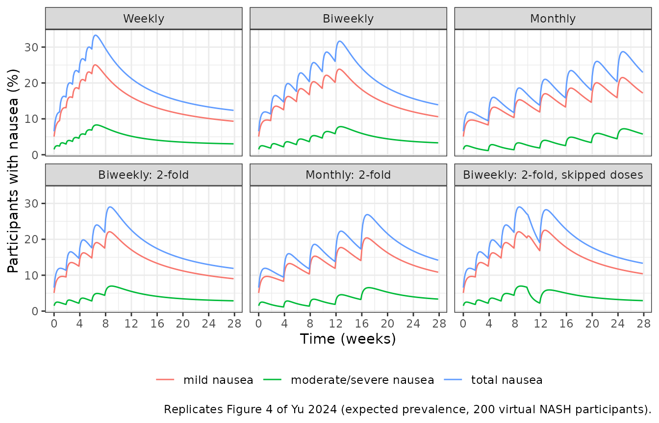
The paper quotes the total-nausea level at 600 ug for four scenarios, and the off-drug trough and the rebound for the skipped-dose scenario. The table compares them with the peak of the simulated mean after the step to 600 ug (the trough and rebound are the minimum during, and the peak after, the two weeks off drug).
peak_600 <- fig4 |>
  filter(dose_ug == 600) |>
  group_by(scenario) |>
  summarise(simulated = 100 * max(total), .groups = "drop")
skip_prev <- fig4 |> filter(scenario == "Biweekly: 2-fold, skipped doses")
skip_trough <- 100 * min(skip_prev$total[skip_prev$day %in% 71:84])
skip_rebound <- 100 * max(skip_prev$total[skip_prev$day >= 85])

fig4_cmp <- tibble::tribble(
  ~quantity, ~scenario, ~published,
  "Peak at 600 ug", "Weekly", 30,
  "Peak at 600 ug", "Biweekly: 2-fold", 25,
  "Peak at 600 ug", "Monthly", 22.4,
  "Peak at 600 ug", "Monthly: 2-fold", 21.2,
  "Off-drug trough", "Biweekly: 2-fold, skipped doses", 10,
  "Rebound on resumption", "Biweekly: 2-fold, skipped doses", 21
) |>
  left_join(mutate(peak_600, quantity = "Peak at 600 ug", scenario = as.character(scenario)),
    by = c("quantity", "scenario")
  ) |>
  mutate(simulated = case_when(
    quantity == "Off-drug trough" ~ skip_trough,
    quantity == "Rebound on resumption" ~ skip_rebound,
    TRUE ~ simulated
  ))
fig4_cmp |>
  dplyr::rename(
    "Quantity" = quantity, "Scenario" = scenario,
    "Published (%)" = published, "Simulated (%)" = simulated
  ) |>
knitr::kable(digits = 1)| Quantity | Scenario | Published (%) | Simulated (%) |
|---|---|---|---|
| Peak at 600 ug | Weekly | 30.0 | 33.3 |
| Peak at 600 ug | Biweekly: 2-fold | 25.0 | 29.0 |
| Peak at 600 ug | Monthly | 22.4 | 28.7 |
| Peak at 600 ug | Monthly: 2-fold | 21.2 | 26.9 |
| Off-drug trough | Biweekly: 2-fold, skipped doses | 10.0 | 19.1 |
| Rebound on resumption | Biweekly: 2-fold, skipped doses | 21.0 | 28.3 |
The skipped-dose trough is the largest miss. With the packaged clock, which resets on any change of the daily dose as in the control stream, stopping the drug restarts the tolerance clock of the 0 -> {1,2} transition and new mild episodes keep appearing while mild nausea resolves at only a few percent per day. The paper’s Methods describe the clock as the time since the last dose escalation; a clock that ignores the step down to no dose and restarts only on the resumption gives the values below, a little closer to the figure but still well above its 10% trough.
days_since_escalation <- function(dose_ug) {
  escalated <- dose_ug > c(0, utils::head(dose_ug, -1))
  last <- cummax(ifelse(escalated, seq_along(dose_ug), 0L))
  seq_along(dose_ug) - last
}
ev_esc <- markov_events(cohort_nash, skip, "escalation clock")
ev_esc$T_DOSECHANGE <- 24 * days_since_escalation(skip)[ev_esc$day]
sim_esc <- as.data.frame(rxode2::rxSolve(mod_typ, ev_esc, returnType = "data.frame"))
#> ℹ omega/sigma items treated as zero: 'etaslp_t_0', 'etabl_01', 'etabl_10', 'etabl_20'
prev_esc <- prevalence(propagate(sim_esc, n_days))
data.frame(
  clock = c("Any dose change (packaged)", "Escalations only"),
  trough = c(skip_trough, 100 * min(prev_esc$total[prev_esc$day %in% 71:84])),
  rebound = c(skip_rebound, 100 * max(prev_esc$total[prev_esc$day >= 85]))
) |>
  dplyr::rename(
    "Tolerance clock" = clock, "Off-drug trough (%)" = trough,
    "Rebound (%)" = rebound
  ) |>
knitr::kable(digits = 1)| Tolerance clock | Off-drug trough (%) | Rebound (%) |
|---|---|---|
| Any dose change (packaged) | 19.1 | 28.3 |
| Escalations only | 16.2 | 27.0 |
peaks <- stats::setNames(peak_600$simulated, as.character(peak_600$scenario))
quoted <- fig4_cmp$quantity != "Off-drug trough"
stopifnot(
  # Weekly steps give the highest peak of the four quoted, as in the paper.
  peaks[["Weekly"]] > peaks[["Biweekly: 2-fold"]],
  peaks[["Weekly"]] > peaks[["Monthly: 2-fold"]],
  # Level: a mis-scaled AUC (dose in mg instead of ug) or a tolerance slope
  # read per hour moves these peaks by a factor of two or more. The trough is
  # left out (see above).
  all(abs(fig4_cmp$simulated[quoted] / fig4_cmp$published[quoted] - 1) < 0.5),
  # Skipping doses lowers nausea and resuming brings it back.
  skip_trough < 0.8 * peaks[["Biweekly: 2-fold, skipped doses"]],
  skip_rebound > 1.2 * skip_trough
)
Covariate effects (Figure 3)
Figure 3 gives the nausea prevalence at 600 ug of males, obesity and NASH participants relative to female T2DM participants. The paper does not state the simulated regimen; it is taken here as the biweekly two-fold titration, with the prevalence averaged over the first seven days at 600 ug, the window the paper uses for its observed rates (Appendix S1 Figure S1). All four arms share the same random effects.
arms <- list(
  "Reference (T2DM female)" = c(SEXF = 1, DIS_OBESE = 0, DIS_NASH = 0),
  "Sex: male" = c(SEXF = 0, DIS_OBESE = 0, DIS_NASH = 0),
  "IND: Obesity" = c(SEXF = 1, DIS_OBESE = 1, DIS_NASH = 0),
  "IND: NASH" = c(SEXF = 1, DIS_OBESE = 0, DIS_NASH = 1)
)
bw2 <- scenarios[["Biweekly: 2-fold"]]
window <- which(bw2 == 600)[1:7]
fig3 <- bind_rows(lapply(names(arms), function(a) {
  coh <- cohort_nash
  coh$SEXF <- arms[[a]][["SEXF"]]
  coh$DIS_OBESE <- arms[[a]][["DIS_OBESE"]]
  coh$DIS_NASH <- arms[[a]][["DIS_NASH"]]
  ev <- markov_events(coh, bw2, a)
  sim <- as.data.frame(rxode2::rxSolve(mod_typ, ev, returnType = "data.frame"))
  prevalence(propagate(sim, n_days)) |>
    filter(day %in% window) |>
    summarise(total = mean(total), mild = mean(mild), severe = mean(severe)) |>
    mutate(arm = a)
}))
#> ℹ omega/sigma items treated as zero: 'etaslp_t_0', 'etabl_01', 'etabl_10', 'etabl_20'
#> ℹ omega/sigma items treated as zero: 'etaslp_t_0', 'etabl_01', 'etabl_10', 'etabl_20'
#> ℹ omega/sigma items treated as zero: 'etaslp_t_0', 'etabl_01', 'etabl_10', 'etabl_20'
#> ℹ omega/sigma items treated as zero: 'etaslp_t_0', 'etabl_01', 'etabl_10', 'etabl_20'
ref <- fig3[1, ]
fig3_ratio <- fig3 |>
  mutate(total = total / ref$total, mild = mild / ref$mild, severe = severe / ref$severe)

# Ratios digitised by the maintainers from Figure 3.
fig3_pub <- tibble::tribble(
  ~arm, ~total, ~mild, ~severe,
  "Reference (T2DM female)", 1, 1, 1,
  "Sex: male", 0.78, 0.80, 0.78,
  "IND: Obesity", 0.67, 0.52, 0.97,
  "IND: NASH", 1.02, 1.15, 0.78
)
fig3_both <- bind_rows(
  mutate(fig3_ratio, source = "Simulated"),
  mutate(fig3_pub, source = "Published (Figure 3)")
) |>
  pivot_longer(c(total, mild, severe), names_to = "nausea", values_to = "ratio") |>
  mutate(
    nausea = factor(recode(nausea,
      total = "Total nausea", mild = "Mild nausea",
      severe = "Moderate/severe nausea"
    ), levels = c("Total nausea", "Mild nausea", "Moderate/severe nausea")),
    arm = factor(arm, levels = rev(names(arms)))
  )
ggplot(fig3_both, aes(ratio, arm, shape = source, colour = source)) +
  geom_vline(xintercept = 1) +
  geom_point(size = 2.5) +
  facet_wrap(~nausea) +
  labs(
    x = "Ratio to reference", y = NULL, shape = NULL, colour = NULL,
    caption = "Replicates Figure 3 of Yu 2024."
  ) +
  theme_bw() +
  theme(legend.position = "bottom")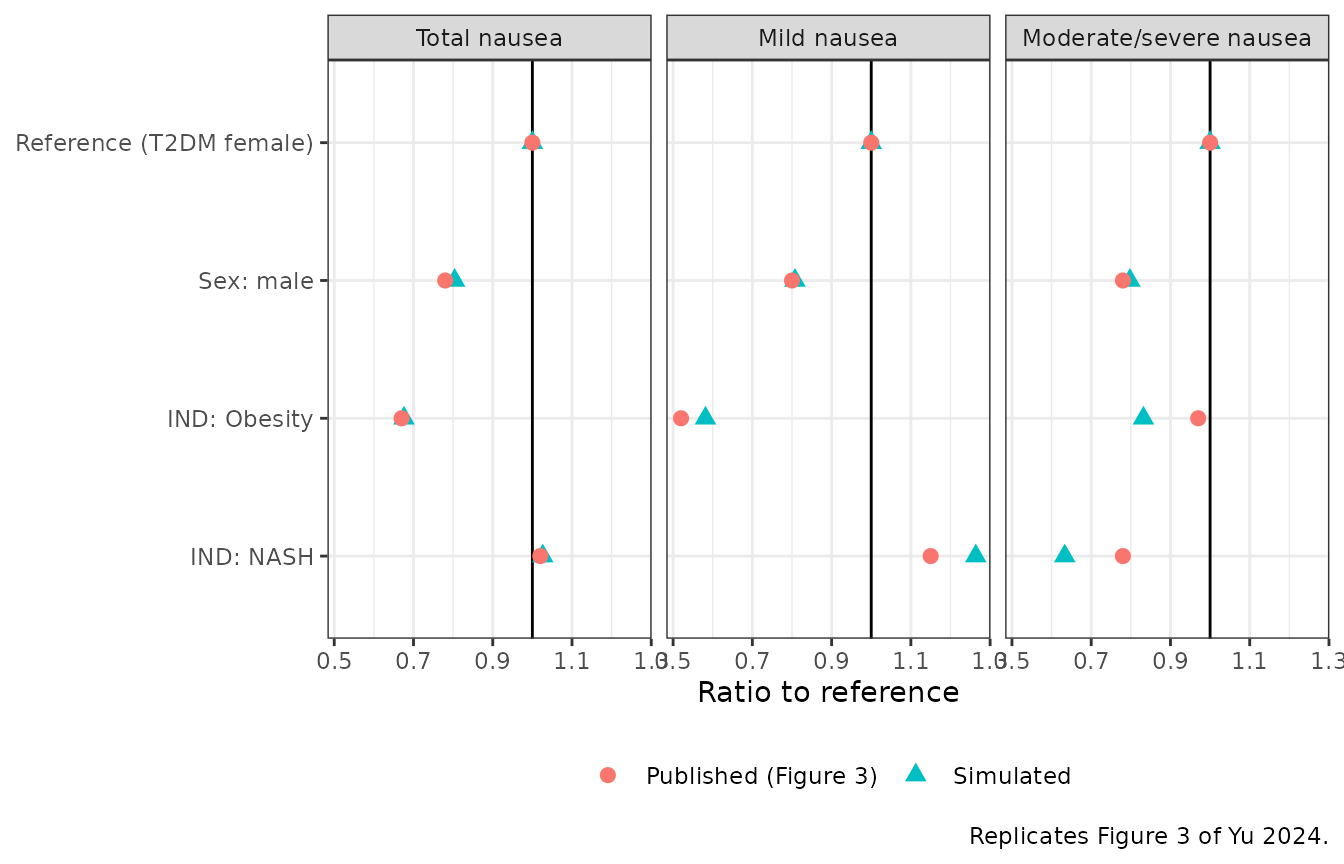
fig3_ratio |>
  select(arm, total, mild, severe) |>
  dplyr::rename(
    "Arm" = arm, "Total" = total, "Mild" = mild,
    "Moderate/severe" = severe
  ) |>
knitr::kable(digits = 2)| Arm | Total | Mild | Moderate/severe |
|---|---|---|---|
| Reference (T2DM female) | 1.00 | 1.00 | 1.00 |
| Sex: male | 0.80 | 0.81 | 0.80 |
| IND: Obesity | 0.68 | 0.58 | 0.83 |
| IND: NASH | 1.03 | 1.26 | 0.63 |
sim_r <- fig3_ratio |> filter(arm != "Reference (T2DM female)")
pub_r <- fig3_pub |> filter(arm != "Reference (T2DM female)")
stopifnot(
  # The sex effect is a plain additive logit shift, so its ratio is close
  # to the paper's 0.78-0.80 for every severity.
  all(abs(unlist(sim_r[sim_r$arm == "Sex: male", c("total", "mild", "severe")]) - 0.79) < 0.1),
  # Total and mild nausea: obesity lowers them, NASH leaves total nausea about
  # unchanged; a wrong sign or a beta effect read as additive moves these by
  # 0.3 or more.
  all(abs(sim_r$total - pub_r$total) < 0.15),
  all(abs(sim_r$mild - pub_r$mild) < 0.2)
)
Sampled Markov chain
The probabilities above are exact expectations over the chain. A sampled chain with the same random effects, using base R uniform draws, must agree with them up to Monte Carlo error, and gives the number of transitions between states, the quantity of the paper’s posterior predictive check (Figure 2).
ev <- markov_events(cohort_nash, bw2, "Biweekly: 2-fold")
sim_bw2 <- as.data.frame(rxode2::rxSolve(mod_typ, ev, returnType = "data.frame"))
#> ℹ omega/sigma items treated as zero: 'etaslp_t_0', 'etabl_01', 'etabl_10', 'etabl_20'
set.seed(42)
u <- matrix(stats::runif(n_sub * n_days), n_sub, n_days)
st <- sample_chain(sim_bw2, n_days, u)
exact <- prevalence(propagate(sim_bw2, n_days))
chain_prev <- data.frame(week = (seq_len(n_days) - 1) / 7, sampled = colMeans(st > 0))

ggplot(exact, aes(week, 100 * total)) +
  geom_line(aes(colour = "Exact expectation")) +
  geom_line(data = chain_prev, aes(week, 100 * sampled, colour = "Sampled chain")) +
  labs(
    x = "Time (weeks)", y = "Participants with nausea (%)", colour = NULL,
    caption = "Biweekly two-fold titration, 200 virtual NASH participants."
  ) +
  theme_bw()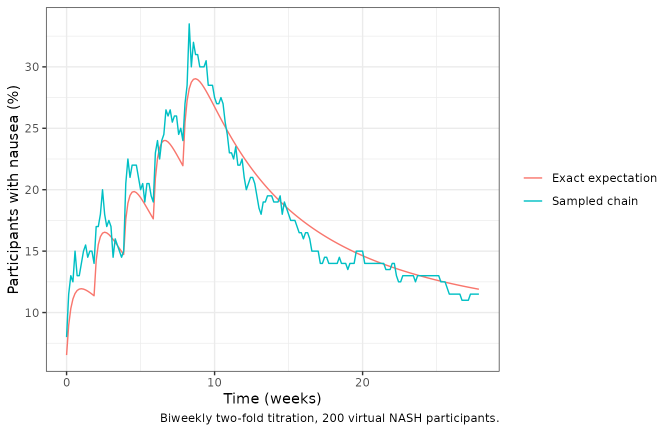
trans <- table(
  from = factor(st[, -n_days], levels = 0:2),
  to = factor(st[, -1], levels = 0:2)
)
trans
#>     to
#> from     0     1     2
#>    0 31827   175    70
#>    1   170  5508     0
#>    2    68     0  1182

# The sampled mean scatters around the exact expectation by about
# sqrt(0.2 * 0.8 / 200) = 3 percentage points per day; averaged over all days
# the difference is far smaller.
stopifnot(abs(mean(chain_prev$sampled - exact$total)) < 0.02)
The Figure 2 check was run on cohort 3 of study D5670C00004 (300 ug after weekly 100 ug steps, T2DM). The cohort size and follow-up are not given, so its transition counts are not reproduced here.
Assumptions and deviations
-
Indication effects on the tolerance slope. Table 3
places the NASH (-0.58) and obesity (-0.75) effects on beta 1,2|0, the
slope that carries the exponential random effect, while the Results text
says the indications act on the baselines. No covariate equation is
printed. The maintainers compared candidate forms by simulation against
Figures 3 and 4: an additive shift of the baseline (the text) or of the
slope gives total-nausea ratios of about 0.3 for obesity and 0.6 for
NASH against the plotted 0.67 and 1.0 and was rejected;
beta * exp(theta)andbeta * (1 + theta)both come close, with the exponential form matching the total and mild ratios and the Figure 4 levels better. The model usesslp_t_0 * exp(e_nash_slp_t_0 * DIS_NASH + e_obese_slp_t_0 * DIS_OBESE + etaslp_t_0). -
Covariate effects on the baselines (sex, obesity,
NASH) are additive on the logit. A multiplicative
BL * (1 + theta)form gives a male ratio near 1.8 against the plotted 0.78; the additive form reproduces it. -
Sex. Table 3’s sex effect is applied to males
(
1 - SEXF): the forest plot’s reference is ‘T2DM female’ and the Results report males with a 24% lower nausea rate. -
Random-effect variances are
log(1 + CV^2)from the Table 3 %CV, per its footnote. The base control stream in Appendix S1 also lists random effects on the three AUC slopes and on the other two tolerance slopes; the final model in Table 3 keeps only the four listed here. - PK layer. The paper drove the nausea model with each participant’s post hoc CL/F from the upstream population PK model (which has covariates for body weight, ADA titre, indication, ALT, formulation and device). That model’s parameters are not printed in Yu 2024, so the packaged model uses the typical CL/F of 1.05 L/h for everyone. Simulated nausea in a population whose CL/F differs systematically from 1.05 L/h will differ from the paper’s.
- Figure 4 levels. The simulated peaks run above the quoted 30%, 25%, 22.4% and 21.2% (see the table above). Plausible contributors are the typical-CL/F PK layer (the upstream model has an indication effect on CL/F), the unstated sex mix of the simulated NASH population and the unprinted form of the indication effects; the parameters were not adjusted.
- Figure 3 regimen. The regimen behind Figure 3 is not stated; the biweekly two-fold titration and the first week at 600 ug are assumptions. The moderate/severe ratios for obesity and NASH agree less well than the total and mild ratios.
-
Tolerance clock.
T_DOSECHANGEfollows the control stream: it resets whenever the record’s dose value changes, including on a skipped day and on resumption, and is 0 on the first treatment day. The Methods text calls it the time since the last dose escalation; the two readings differ only when the dose goes down or stops. Neither reproduces the sharp drop to 10% during the two weeks off drug in Figure 4 (simulated troughs of about 16-19%); the rebound on resumption is reproduced in direction. - Vomiting was not modelled by the authors and is not included.