Testosterone undecanoate (Pastuszak 2021) • nlmixr2lib

Model and source

Citation: Pastuszak AW, Bush M, Curd L, Vijayan S, Priestley T, Xiang Q, Hu Y. Population Pharmacokinetic Modeling and Simulations to Evaluate a Potential Dose Regimen of Testosterone Undecanoate in Hypogonadal Males. J Clin Pharmacol 2021;61(12):1618-1625. doi:10.1002/jcph.1939.
Description: One-compartment population PK model for total serum testosterone after intramuscular testosterone undecanoate 750 mg in adult men with hypogonadism, with first-order absorption from the injection depot, linear apparent clearance, and an apparent zero-order endogenous testosterone input into the central compartment that is acutely suppressed from its predose rate after the first injection and then recovers gradually to a steady-state rate. Body weight scales CL/F (fixed allometric 0.75), V/F (fixed 1) and Ka (estimated -1.83); baseline sex hormone-binding globulin scales CL/F.
Article (open access): https://doi.org/10.1002/jcph.1939

The model describes total serum testosterone after 750 mg intramuscular testosterone undecanoate (Aveed) in men with hypogonadism. Testosterone undecanoate is absorbed slowly from the oily intramuscular depot (absorption half-life about 29 days at 101 kg), and the model adds an apparent zero-order endogenous testosterone input into the central compartment:

$R(t) = R_b e^{-K_1 t} + R_{ss}\left(1 - e^{-K_2 t}\right)$

R_b (kin_te) is the predose production rate. It is switched off within hours of the first injection (K_1 = 10 1/h, fixed) and then recovers, with a half-life of about 40 days, to the steady-state rate R_ss (kin_te_ss).

Population

The model was fitted to 2360 total testosterone concentrations from 130 men with hypogonadism in the phase 3, single-arm, open-label Study IP157-001 Part C (NCT00467870), run at 31 US sites (Pastuszak 2021 Methods and Table 1). Mean age was 54.2 years (range 24-75), mean weight 101.2 kg (SD 18.0), mean BMI 32.0 kg/m^2 and mean baseline SHBG 20.9 nmol/L (SD 8.9); 74.6% were White, 12.3% Black and 13.1% other races. Patients received 750 mg in 3 mL of castor oil and benzyl benzoate into the buttock at baseline, week 4 and then every 10 weeks for up to 84 weeks. Sampling was dense across injection intervals 3 and 4 (weeks 14-34). The 117-patient original-study PK population (mean weight 101.6 kg, SD 17.4; mean SHBG 20.8 nmol/L, SD 8.5) was the template for the paper’s simulations.

The same information is available programmatically:

str(rxode2::rxode(readModelDb("Pastuszak_2021_testosteroneUndecanoate"))$population)
#> ℹ parameter labels from comments will be replaced by 'label()'
#> List of 14
#>  $ species       : chr "human"
#>  $ n_subjects    : int 130
#>  $ n_studies     : int 1
#>  $ n_observations: int 2360
#>  $ age_range     : chr "24-75 years (enrolled); 30-75 years (PK population)"
#>  $ age_mean      : chr "54.2 years (enrolled); 54.6 years (PK population)"
#>  $ weight_mean   : chr "101.2 kg (SD 18.0) enrolled; 101.6 kg (SD 17.4) PK population"
#>  $ sex_female_pct: num 0
#>  $ race_ethnicity: Named num [1:3] 74.6 12.3 13.1
#>   ..- attr(*, "names")= chr [1:3] "White" "Black" "Other"
#>  $ disease_state : chr "adult men with hypogonadism (primary or hypogonadotropic)"
#>  $ dose_range    : chr "testosterone undecanoate 750 mg in 3 mL castor oil / benzyl benzoate intramuscularly into the buttock at baseli"| __truncated__
#>  $ regions       : chr "United States (31 sites)"
#>  $ shbg_mean     : chr "20.9 nmol/L (SD 8.9) enrolled; 20.8 nmol/L (SD 8.5) PK population"
#>  $ notes         : chr "Phase 3 single-arm open-label Study IP157-001 Part C (NCT00467870); Table 1. Dense sampling across injection in"| __truncated__

Source trace

Equation / parameter	Value	Source location
`lka` (Ka at 101 kg)	0.001 1/h	Table 2 (units printed ‘L/h’)
`lcl` (CL/F at 101 kg, SHBG 20 nmol/L)	197 L/h	Table 2
`lvc` (V/F at 101 kg)	12 300 L	Table 2
`lkin_te` (Rb)	0.445 mg/h	Table 2
`lkin_te_ss` (Rss)	0.572 mg/h	Table 2
`lk_suppression_te` (K1)	10 1/h, fixed	Table 2 (units printed ‘L/h’)
`lk_recovery_te` (K2)	0.000727 1/h	Table 2 (units printed ‘L/h’)
`e_wt_cl`	0.75, fixed	Table 2
`e_sex_hormone_binding_globulin_cl`	-0.219	Table 2
`e_wt_ka`	-1.83	Table 2
`e_wt_vc`	1, fixed	Table 2
Reference covariate values	101 kg, 20 nmol/L	Table 2 footnote b
`etalcl`	0.0392 (20.0% CV)	Table 2; `log(CV^2 + 1)`
`etalka`	0.2004 (47.1% CV)	Table 2; `log(CV^2 + 1)`
No IIV on V/F	n/a	Results (‘The model did not support estimation of interindividual variability on V/F’)
`propSd`	0.188	Table 2
`addSd`	56.8 ng/dL	Table 2
Structure: 1 compartment, first-order absorption and elimination	n/a	Results; Figure 1
`R(t)` endogenous input equation	n/a	Results, equation following Figure 1
Covariate forms: power models centred on the reference values	n/a	Methods (Population PK Modeling); Table 2
`central(0) <- kin_te / kel`	n/a	Assumed: predose endogenous steady state (see Assumptions)
`Cc <- central / vc * 1e5` (mg/L to ng/dL)	n/a	Unit conversion; concentrations in ng/dL throughout

Virtual cohort

Observed data are not public. As in the paper, each regimen is simulated in a cohort of 117 men whose covariates follow the PK population in Table 1. The same 117 covariate sets are used for both regimens. Weight is normal (mean 101.6 kg, SD 17.4) with a floor of 65 kg, the study’s PK-population inclusion threshold. SHBG is log-normal with mean 20.8 nmol/L and SD 8.5.

Dosing is 750 mg at week 0, at week 4, and then every 10 weeks (approved) or every 8 weeks (alternative), through dose 10. As in the paper, concentrations are sampled every 48 hours.

n_sub <- 117L
h_per_week <- 168

cov <- tibble(
  sub = seq_len(n_sub),
  WT = pmax(65, rnorm(n_sub, 101.6, 17.4)),
  SEX_HORMONE_BINDING_GLOBULIN = {
    sdl <- sqrt(log(1 + (8.5 / 20.8)^2))
    exp(rnorm(n_sub, log(20.8) - sdl^2 / 2, sdl))
  }
)

dose_weeks <- function(tau_weeks) c(0, 4, 4 + tau_weeks * (1:8))

make_cohort <- function(tau_weeks, id_offset) {
  dose_t <- dose_weeks(tau_weeks) * h_per_week
  end_t <- dose_t[10] + tau_weeks * h_per_week
  obs_t <- seq(0, end_t, by = 48)
  per_sub <- function(i) {
    dplyr::bind_rows(
      tibble(time = dose_t, amt = 750, evid = 1L, cmt = "depot"),
      tibble(time = obs_t, amt = 0, evid = 0L, cmt = "central")
    ) |>
      dplyr::mutate(
        id = id_offset + i,
        WT = cov$WT[i],
        SEX_HORMONE_BINDING_GLOBULIN = cov$SEX_HORMONE_BINDING_GLOBULIN[i]
      )
  }
  dplyr::bind_rows(lapply(seq_len(n_sub), per_sub)) |>
    dplyr::mutate(regimen = paste0("Q", tau_weeks, "W"), tau_weeks = tau_weeks) |>
    dplyr::arrange(id, time, dplyr::desc(evid))
}

events <- dplyr::bind_rows(
  make_cohort(10, id_offset = 0L),
  make_cohort(8, id_offset = 1000L)
)
stopifnot(!anyDuplicated(unique(events[, c("id", "time", "evid")])))

Simulation

mod <- readModelDb("Pastuszak_2021_testosteroneUndecanoate")
sim <- rxode2::rxSolve(mod, events = events, keep = c("regimen", "tau_weeks")) |>
  as.data.frame()
#> ℹ parameter labels from comments will be replaced by 'label()'

The paper’s simulated exposure metrics include residual variability, so the per-patient Cmax, Cavg and Ctrough below are computed from the sim column (the prediction with residual error added), not from Cc (the individual prediction).

Replicate published figures

Figure 2: concentration-time profile under the approved regimen

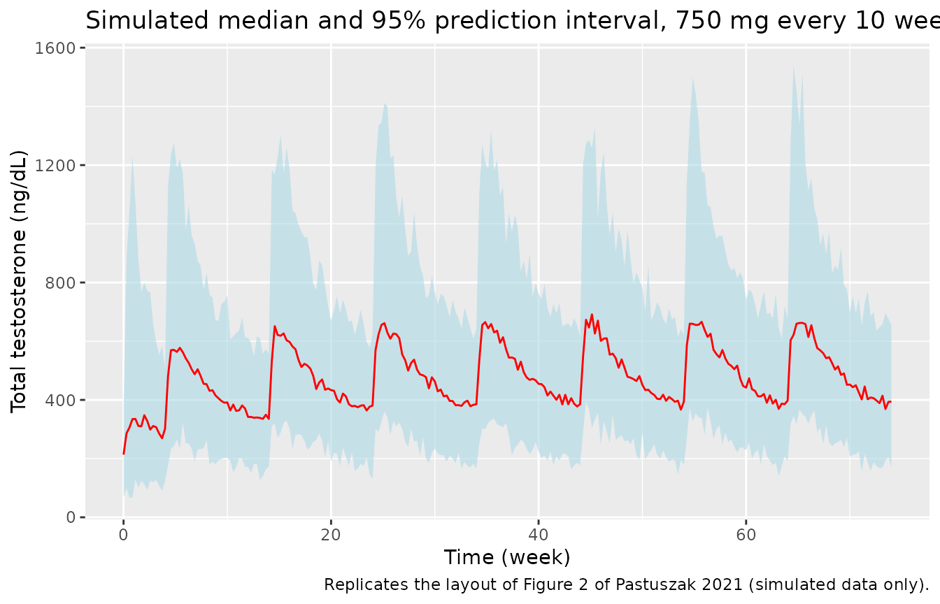
Figure 2 of the paper is a prediction-corrected VPC of the observed data. The observations are not public, so the plot below shows the simulated median and 95% prediction interval for the approved regimen over the same 0-74 week window. It reproduces the paper’s shape: a predose baseline near 230 ng/dL, a drop then rise over the first two injections, peaks near 1000 ng/dL after each injection, and troughs that rise slowly as endogenous production recovers.

sim |>
  dplyr::filter(regimen == "Q10W", time <= 74 * h_per_week) |>
  dplyr::group_by(time) |>
  dplyr::summarise(
    lo = quantile(sim, 0.025),
    med = median(sim),
    hi = quantile(sim, 0.975),
    .groups = "drop"
  ) |>
  ggplot(aes(time / h_per_week, med)) +
  geom_ribbon(aes(ymin = lo, ymax = hi), fill = "lightblue", alpha = 0.6) +
  geom_line(colour = "red") +
  labs(
    x = "Time (week)", y = "Total testosterone (ng/dL)",
    title = "Simulated median and 95% prediction interval, 750 mg every 10 weeks",
    caption = "Replicates the layout of Figure 2 of Pastuszak 2021 (simulated data only)."
  )

Typical-value check against Table 4

Typical-value Cavg after dose 10 depends only on clearance, dose and the endogenous input, so it tests the structural model, the dose and the units directly. It is computed for a 101 kg patient with SHBG 20 nmol/L. Only Cavg is compared here: the paper’s Cmax and Ctrough include residual error, which shifts them away from the typical-value prediction.

mod_typ <- rxode2::zeroRe(mod)
#> ℹ parameter labels from comments will be replaced by 'label()'
# One single-subject solve per regimen for the typical patient.
solve_typical <- function(tau_weeks) {
  ev <- make_cohort(tau_weeks, id_offset = 0L) |>
    dplyr::filter(id == 1) |>
    dplyr::mutate(WT = 101, SEX_HORMONE_BINDING_GLOBULIN = 20)
  rxode2::rxSolve(mod_typ, events = ev, keep = c("regimen", "tau_weeks")) |>
    as.data.frame()
}
sim_typ <- dplyr::bind_rows(solve_typical(10), solve_typical(8))
#> ℹ omega/sigma items treated as zero: 'etalcl', 'etalka'
#> ℹ omega/sigma items treated as zero: 'etalcl', 'etalka'

typ_cavg <- sim_typ |>
  dplyr::group_by(regimen, tau_weeks) |>
  dplyr::summarise(
    cavg = {
      start <- dose_weeks(tau_weeks[1])[10] * h_per_week
      end <- start + tau_weeks[1] * h_per_week
      keep <- time >= start & time <= end
      tt <- time[keep]
      cc <- Cc[keep]
      sum(diff(tt) * (head(cc, -1) + tail(cc, -1)) / 2) / (end - start)
    },
    .groups = "drop"
  ) |>
  dplyr::mutate(published = c(Q10W = 510.1, Q8W = 564.5)[regimen])

typ_cavg |>
  dplyr::mutate(pct_diff = 100 * (cavg / published - 1)) |>
  dplyr::rename(
    "Regimen" = regimen,
    "Typical-value Cavg (ng/dL)" = cavg,
    "Table 4 median Cavg (ng/dL)" = published,
    "% diff" = pct_diff
  ) |>
  dplyr::select(-tau_weeks) |>
  knitr::kable(digits = 1, caption = "Typical-value Cavg after dose 10 vs. Pastuszak 2021 Table 4.")

Typical-value Cavg after dose 10 vs. Pastuszak 2021 Table 4.
Regimen	Typical-value Cavg (ng/dL)	Table 4 median Cavg (ng/dL)	% diff
Q10W	516.3	510.1	1.2
Q8W	572.7	564.5	1.5


# Predose baseline is the endogenous steady state Rb / CL.
baseline_typ <- sim_typ$Cc[sim_typ$time == 0 & sim_typ$regimen == "Q10W"][1]
baseline_closed <- 0.445 / 197 * 1e5

cavg_ratio <- typ_cavg$cavg[typ_cavg$regimen == "Q8W"] /
  typ_cavg$cavg[typ_cavg$regimen == "Q10W"]

stopifnot(
  # Solve against its own closed form: numerical error only.
  abs(baseline_typ / baseline_closed - 1) < 1e-4,
  # Deterministic; realised +1.2% (Q10W) and +1.5% (Q8W). A wrong dose,
  # clearance or unit conversion moves Cavg by tens of percent.
  all(abs(typ_cavg$cavg / typ_cavg$published - 1) < 0.05),
  # Table 4 Cavg ratio 1.11; realised 1.109 (deterministic).
  abs(cavg_ratio - 1.11) < 0.03
)

PKNCA validation

Cmax, Cavg and Ctrough are computed per patient for each dosing interval with PKNCA, using the sim concentrations sampled every 48 hours. The paper defines Ctrough as the last observed concentration in the dosing interval before the next dose, which is PKNCA’s clast.obs. Dose 1 covers weeks 0-4, so its interval is 4 weeks for both regimens.

dose_df <- events |>
  dplyr::filter(evid == 1) |>
  dplyr::select(id, time, amt, regimen)
dose_obj <- PKNCA::PKNCAdose(dose_df, amt ~ time | regimen + id)

interval_tbl <- dplyr::bind_rows(lapply(c(10, 8), function(tau) {
  dt <- dose_weeks(tau) * h_per_week
  tibble(
    regimen = paste0("Q", tau, "W"),
    dose_number = c(1, 2, 3, 4, 10),
    start = dt[c(1, 2, 3, 4, 10)],
    end = c(dt[2], dt[c(3, 4, 5)], dt[10] + tau * h_per_week)
  )
}))

intervals <- interval_tbl |>
  dplyr::select(regimen, start, end) |>
  dplyr::mutate(cmax = TRUE, cav = TRUE, clast.obs = TRUE) |>
  as.data.frame()

run_nca <- function(sim_df) {
  # Residual error can push a few low simulated observations below zero; an
  # assay cannot report a negative concentration, so they are floored at 0.
  sim_nca <- sim_df |>
    dplyr::filter(!is.na(sim)) |>
    dplyr::mutate(Cc = pmax(sim, 0)) |>
    dplyr::select(id, time, Cc, regimen)
  conc_obj <- PKNCA::PKNCAconc(sim_nca, Cc ~ time | regimen + id)
  # Linear trapezoids: Cavg is the time-average of the 48-hour samples.
  nca_data <- PKNCA::PKNCAdata(
    conc_obj, dose_obj,
    intervals = intervals,
    options = list(auc.method = "linear")
  )
  out <- as.data.frame(PKNCA::pk.nca(nca_data)) |>
    dplyr::left_join(interval_tbl, by = c("regimen", "start", "end"))
  stopifnot(
    !anyNA(out$dose_number),
    !anyNA(out$PPORRES[out$PPTESTCD %in% c("cmax", "cav", "clast.obs")])
  )
  out
}

nca_long <- run_nca(sim)

Comparison against Table 4 (dose 10)

Table 4 reports, for each exposure metric, the median over 500 simulated studies of the per-study median. In the table below, Ctrough is the row labelled Clast (PKNCA’s clast.obs).

published <- tibble::tribble(
  ~regimen, ~cmax, ~cav, ~clast.obs,
  "Q8W", 978.2, 564.5, 391.3,
  "Q10W", 934.2, 510.1, 351.9
)

sim_dose10 <- nca_long |>
  dplyr::filter(dose_number == 10, PPTESTCD %in% c("cmax", "cav", "clast.obs")) |>
  dplyr::select(id, regimen, PPTESTCD, PPORRES)

cmp <- nlmixr2lib::ncaComparisonTable(
  simulated = sim_dose10,
  reference = published,
  by = "regimen",
  units = c(cmax = "ng/dL", cav = "ng/dL", clast.obs = "ng/dL"),
  tolerance_pct = 20
)
knitr::kable(
  cmp,
  caption = "Simulated vs. Pastuszak 2021 Table 4 (dose 10). * differs from reference by >20%."
)

Simulated vs. Pastuszak 2021 Table 4 (dose 10). * differs from reference by >20%.
NCA parameter	regimen	Reference	Simulated	% diff
Cmax (ng/dL)	Q8W	978	921	-5.9%
Cmax (ng/dL)	Q10W	934	849	-9.1%
Clast (ng/dL)	Q8W	391	430	+9.8%
Clast (ng/dL)	Q10W	352	365	+3.6%
Cavg (ng/dL)	Q8W	564	553	-2.1%
Cavg (ng/dL)	Q10W	510	517	+1.4%


med10 <- sim_dose10 |>
  dplyr::group_by(regimen, PPTESTCD) |>
  dplyr::summarise(med = median(PPORRES), .groups = "drop") |>
  dplyr::left_join(
    tidyr::pivot_longer(published, -regimen, names_to = "PPTESTCD", values_to = "ref"),
    by = c("regimen", "PPTESTCD")
  )
stopifnot(nrow(med10) == 6L)
med10
#> # A tibble: 6 × 4
#>   regimen PPTESTCD    med   ref
#>   <chr>   <chr>     <dbl> <dbl>
#> 1 Q10W    cav        517.  510.
#> 2 Q10W    clast.obs  365.  352.
#> 3 Q10W    cmax       849.  934.
#> 4 Q8W     cav        553.  564.
#> 5 Q8W     clast.obs  430.  391.
#> 6 Q8W     cmax       921.  978.
stopifnot(
  # Cavg is structural (dose, CL, endogenous input); realised within 2%.
  all(abs(med10$med[med10$PPTESTCD == "cav"] / med10$ref[med10$PPTESTCD == "cav"] - 1) < 0.10),
  # Cmax and Ctrough of one 117-patient cohort, also shifted by the rounding
  # of Ka in Table 2 (see Assumptions): realised within 10%. A wrong dose,
  # volume or unit moves them by far more than 25%.
  all(abs(med10$med / med10$ref - 1) < 0.25)
)

Simulated Cavg agrees with Table 4 to within a few percent for both regimens. Median Cmax tends to come out low (about 5-10%) and median Ctrough high (up to about 10%). That is the pattern expected if Ka is slightly too small, and Table 2 prints Ka to only one significant figure (see the sensitivity run below).

Percentage of patients within the prespecified ranges (Table 5 and Table S1)

range_summary <- function(nca_df) {
  nca_df |>
  dplyr::filter(PPTESTCD %in% c("cmax", "cav", "clast.obs")) |>
  dplyr::select(id, regimen, dose_number, PPTESTCD, PPORRES) |>
  tidyr::pivot_wider(names_from = PPTESTCD, values_from = PPORRES) |>
  dplyr::group_by(regimen, dose_number) |>
  dplyr::summarise(
    `Cavg 300-1000` = 100 * mean(cav >= 300 & cav <= 1000),
    `Cavg <300` = 100 * mean(cav < 300),
    `Cavg >1000` = 100 * mean(cav > 1000),
    `Cmax <1500` = 100 * mean(cmax < 1500),
    `Cmax 1800-2500` = 100 * mean(cmax >= 1800 & cmax <= 2500),
    `Cmax >2500` = 100 * mean(cmax > 2500),
    `Ctrough >300` = 100 * mean(clast.obs > 300),
    .groups = "drop"
  ) |>
  tidyr::pivot_longer(-c(regimen, dose_number), names_to = "metric", values_to = "simulated")
}
range_tbl <- range_summary(nca_long)

# Table S1 (doses 1-4) and Table 5 (dose 10); medians across 500 simulated studies.
pub_ranges <- tibble::tribble(
  ~metric, ~dose_number, ~Q10W, ~Q8W,
  "Cavg 300-1000", 1, 70.1, 70.1,
  "Cavg 300-1000", 2, 92.3, 94.0,
  "Cavg 300-1000", 3, 96.6, 97.4,
  "Cavg 300-1000", 4, 97.4, 98.3,
  "Cavg 300-1000", 10, 97.4, 98.3,
  "Cavg <300", 1, 29.9, 29.9,
  "Cavg <300", 2, 7.7, 6.0,
  "Cavg <300", 3, 3.4, 1.7,
  "Cavg <300", 4, 2.6, 0.9,
  "Cavg <300", 10, 1.7, 0.9,
  "Cavg >1000", 1, 0.0, 0.0,
  "Cavg >1000", 2, 0.0, 0.0,
  "Cavg >1000", 3, 0.0, 0.0,
  "Cavg >1000", 4, 0.0, 0.9,
  "Cavg >1000", 10, 0.0, 0.9,
  "Cmax <1500", 1, 98.3, 98.3,
  "Cmax <1500", 2, 92.3, 92.3,
  "Cmax <1500", 3, 92.3, 92.3,
  "Cmax <1500", 4, 91.5, 90.6,
  "Cmax <1500", 10, 90.6, 88.9,
  "Cmax 1800-2500", 1, 0.9, 0.9,
  "Cmax 1800-2500", 2, 1.7, 2.6,
  "Cmax 1800-2500", 3, 2.6, 2.6,
  "Cmax 1800-2500", 4, 2.6, 3.4,
  "Cmax 1800-2500", 10, 3.0, 3.4,
  "Cmax >2500", 1, 0.0, 0.0,
  "Cmax >2500", 2, 0.0, 0.0,
  "Cmax >2500", 3, 0.0, 0.0,
  "Cmax >2500", 4, 0.0, 0.0,
  "Cmax >2500", 10, 0.0, 0.0,
  "Ctrough >300", 1, 51.3, 51.3,
  "Ctrough >300", 2, 53.0, 59.8,
  "Ctrough >300", 3, 63.2, 70.1,
  "Ctrough >300", 4, 65.8, 74.4,
  "Ctrough >300", 10, 66.7, 76.1
) |>
  tidyr::pivot_longer(c(Q10W, Q8W), names_to = "regimen", values_to = "published")

range_cmp <- dplyr::inner_join(pub_ranges, range_tbl, by = c("metric", "dose_number", "regimen"))
stopifnot(nrow(range_cmp) == nrow(pub_ranges))

range_cmp |>
  dplyr::arrange(regimen, dose_number) |>
  dplyr::rename(
    "Regimen" = regimen,
    "Dose" = dose_number,
    "Metric (ng/dL)" = metric,
    "Published (%)" = published,
    "Simulated (%)" = simulated
  ) |>
  knitr::kable(digits = 1, caption = "Percentage of patients within each range: Pastuszak 2021 Table S1 (doses 1-4) and Table 5 (dose 10) vs. one simulated 117-patient cohort per regimen.")

Percentage of patients within each range: Pastuszak 2021 Table S1 (doses 1-4) and Table 5 (dose 10) vs. one simulated 117-patient cohort per regimen.
Metric (ng/dL)	Dose	Regimen	Published (%)	Simulated (%)
Cavg 300-1000	1	Q10W	70.1	52.1
Cavg <300	1	Q10W	29.9	47.9
Cavg >1000	1	Q10W	0.0	0.0
Cmax <1500	1	Q10W	98.3	100.0
Cmax 1800-2500	1	Q10W	0.9	0.0
Cmax >2500	1	Q10W	0.0	0.0
Ctrough >300	1	Q10W	51.3	51.3
Cavg 300-1000	2	Q10W	92.3	98.3
Cavg <300	2	Q10W	7.7	1.7
Cavg >1000	2	Q10W	0.0	0.0
Cmax <1500	2	Q10W	92.3	95.7
Cmax 1800-2500	2	Q10W	1.7	0.0
Cmax >2500	2	Q10W	0.0	0.0
Ctrough >300	2	Q10W	53.0	63.2
Cavg 300-1000	3	Q10W	96.6	100.0
Cavg <300	3	Q10W	3.4	0.0
Cavg >1000	3	Q10W	0.0	0.0
Cmax <1500	3	Q10W	92.3	98.3
Cmax 1800-2500	3	Q10W	2.6	0.9
Cmax >2500	3	Q10W	0.0	0.0
Ctrough >300	3	Q10W	63.2	75.2
Cavg 300-1000	4	Q10W	97.4	100.0
Cavg <300	4	Q10W	2.6	0.0
Cavg >1000	4	Q10W	0.0	0.0
Cmax <1500	4	Q10W	91.5	94.9
Cmax 1800-2500	4	Q10W	2.6	0.9
Cmax >2500	4	Q10W	0.0	0.0
Ctrough >300	4	Q10W	65.8	69.2
Cavg 300-1000	10	Q10W	97.4	100.0
Cavg <300	10	Q10W	1.7	0.0
Cavg >1000	10	Q10W	0.0	0.0
Cmax <1500	10	Q10W	90.6	97.4
Cmax 1800-2500	10	Q10W	3.0	1.7
Cmax >2500	10	Q10W	0.0	0.0
Ctrough >300	10	Q10W	66.7	76.1
Cavg 300-1000	1	Q8W	70.1	53.0
Cavg <300	1	Q8W	29.9	46.2
Cavg >1000	1	Q8W	0.0	0.9
Cmax <1500	1	Q8W	98.3	98.3
Cmax 1800-2500	1	Q8W	0.9	1.7
Cmax >2500	1	Q8W	0.0	0.0
Ctrough >300	1	Q8W	51.3	47.0
Cavg 300-1000	2	Q8W	94.0	94.0
Cavg <300	2	Q8W	6.0	6.0
Cavg >1000	2	Q8W	0.0	0.0
Cmax <1500	2	Q8W	92.3	95.7
Cmax 1800-2500	2	Q8W	2.6	1.7
Cmax >2500	2	Q8W	0.0	0.0
Ctrough >300	2	Q8W	59.8	70.1
Cavg 300-1000	3	Q8W	97.4	99.1
Cavg <300	3	Q8W	1.7	0.9
Cavg >1000	3	Q8W	0.0	0.0
Cmax <1500	3	Q8W	92.3	94.9
Cmax 1800-2500	3	Q8W	2.6	1.7
Cmax >2500	3	Q8W	0.0	0.0
Ctrough >300	3	Q8W	70.1	79.5
Cavg 300-1000	4	Q8W	98.3	98.3
Cavg <300	4	Q8W	0.9	0.9
Cavg >1000	4	Q8W	0.9	0.9
Cmax <1500	4	Q8W	90.6	94.9
Cmax 1800-2500	4	Q8W	3.4	2.6
Cmax >2500	4	Q8W	0.0	0.0
Ctrough >300	4	Q8W	74.4	79.5
Cavg 300-1000	10	Q8W	98.3	99.1
Cavg <300	10	Q8W	0.9	0.0
Cavg >1000	10	Q8W	0.9	0.9
Cmax <1500	10	Q8W	88.9	96.6
Cmax 1800-2500	10	Q8W	3.4	2.6
Cmax >2500	10	Q8W	0.0	0.0
Ctrough >300	10	Q8W	76.1	78.6


cavg_in <- range_cmp |>
  dplyr::filter(metric == "Cavg 300-1000", dose_number >= 3)
stopifnot(
  # Paper 96.6-98.3% from dose 3 on; a mis-scaled model drops this far
  # below 85%.
  all(cavg_in$simulated > 85)
)

From dose 2 onwards the Cavg categories match the published percentages closely. Three quantities differ, and all are explained by the rounding of Ka (next section). After dose 1, fewer simulated patients reach a Cavg of 300-1000 ng/dL (about 50-60% against 70.1%), because absorption from the first injection is slower. From dose 2 onwards the share with Ctrough above 300 ng/dL runs up to about 12 points higher than published, and the share with Cmax below 1500 ng/dL up to about 8 points higher.

Sensitivity to the rounding of Ka

Table 2 prints Ka as 0.001 1/h (bootstrap 95% CI 0.001 to 0.002), so any estimate from 0.0005 to 0.0015 would print the same way. The packaged model keeps the printed 0.001. The run below repeats the simulation on the same virtual cohort with Ka = 0.0014 1/h. Faster absorption raises the early (dose 1) exposure and the dose-10 peaks and lowers the dose-10 troughs, which moves every quantity that disagrees above towards the published value, while Cavg after dose 3 is unchanged.

mod_ka <- rxode2::ini(mod, lka = log(0.0014))
#> ℹ parameter labels from comments will be replaced by 'label()'
#> ℹ change initial estimate of `lka` to `-6.57128304236092`
sim_ka <- rxode2::rxSolve(mod_ka, events = events, keep = c("regimen", "tau_weeks")) |>
  as.data.frame()
nca_ka <- run_nca(sim_ka)

ka_medians <- nca_ka |>
  dplyr::filter(dose_number == 10, PPTESTCD %in% c("cmax", "clast.obs")) |>
  dplyr::group_by(regimen, PPTESTCD) |>
  dplyr::summarise(ka_0.0014 = median(PPORRES), .groups = "drop") |>
  dplyr::mutate(metric = paste("Median", ifelse(PPTESTCD == "cmax", "Cmax", "Ctrough"), "(ng/dL), dose 10")) |>
  dplyr::left_join(
    med10 |> dplyr::select(regimen, PPTESTCD, ka_0.001 = med, published = ref),
    by = c("regimen", "PPTESTCD")
  ) |>
  dplyr::select(regimen, metric, published, ka_0.001, ka_0.0014)

ka_ranges <- range_summary(nca_ka) |>
  dplyr::rename(ka_0.0014 = simulated) |>
  dplyr::inner_join(range_cmp, by = c("regimen", "dose_number", "metric")) |>
  dplyr::filter(
    (metric == "Cavg 300-1000" & dose_number == 1) |
      (metric %in% c("Cmax <1500", "Ctrough >300") & dose_number == 10)
  ) |>
  dplyr::mutate(metric = paste0(metric, " (%), dose ", dose_number)) |>
  dplyr::select(regimen, metric, published, ka_0.001 = simulated, ka_0.0014)

dplyr::bind_rows(ka_medians, ka_ranges) |>
  dplyr::arrange(regimen, metric) |>
  dplyr::rename(
    "Regimen" = regimen,
    "Quantity" = metric,
    "Published" = published,
    "Ka 0.001 (packaged)" = ka_0.001,
    "Ka 0.0014 (sensitivity)" = ka_0.0014
  ) |>
  knitr::kable(digits = 1, caption = "Exposure quantities most sensitive to Ka: published values vs. the packaged Ka and Ka = 0.0014 1/h, on the same virtual cohort.")

Exposure quantities most sensitive to Ka: published values vs. the packaged Ka and Ka = 0.0014 1/h, on the same virtual cohort.
Regimen	Quantity	Published	Ka 0.001 (packaged)	Ka 0.0014 (sensitivity)
Q10W	Cavg 300-1000 (%), dose 1	70.1	52.1	67.5
Q10W	Cmax <1500 (%), dose 10	90.6	97.4	88.9
Q10W	Ctrough >300 (%), dose 10	66.7	76.1	61.5
Q10W	Median Cmax (ng/dL), dose 10	934.2	849.3	903.6
Q10W	Median Ctrough (ng/dL), dose 10	351.9	364.5	335.1
Q8W	Cavg 300-1000 (%), dose 1	70.1	53.0	72.6
Q8W	Cmax <1500 (%), dose 10	88.9	96.6	92.3
Q8W	Ctrough >300 (%), dose 10	76.1	78.6	74.4
Q8W	Median Cmax (ng/dL), dose 10	978.2	920.6	975.5
Q8W	Median Ctrough (ng/dL), dose 10	391.3	429.6	367.4

Assumptions and deviations

Ka precision. Table 2 prints Ka to one significant figure (0.001 1/h). The packaged model uses that printed value. With it, simulated Cavg from dose 2 onwards matches Tables 4, 5 and S1. But median Cmax runs low, median Ctrough and the share with Ctrough above 300 ng/dL run high, and too few patients reach the Cavg range after dose 1. Ka = 0.0014 1/h, which also prints as 0.001, moves all of these to the published values. The maintainers checked this in a 600-patient run: dose-1 Cavg 300-1000 ng/dL in 74.5% of patients (published 70.1%), and dose-10 Ctrough above 300 ng/dL in 67.0% (published 66.7%) for the 10-week regimen. The maintainers did not tune Ka, because the unrounded estimate is not published.
Dose amount. The dose is entered as 750 mg of testosterone undecanoate, the labelled amount, with no conversion to testosterone equivalents (474 mg). The paper does not state the dose unit used in the dataset. With 750 mg, typical-value Cavg after dose 10 matches Table 4 to within 2% for both regimens. The testosterone-equivalent dose would give a Cavg near 430 ng/dL. Because CL/F and V/F are apparent parameters, this choice is absorbed into F.
Initial condition. The paper does not print the initial condition. The central compartment starts at the predose endogenous steady state, central(0) = Rb / kel (226 ng/dL for the typical patient). With K1 fixed at 10 1/h, Rb is gone within hours of the first dose. Rb could therefore only have been estimated (8.5% RSE) through the predose baseline it sets, and the Figure 2 VPC median near 230 ng/dL at week 0 agrees.
Time origin. The paper’s TIME in the R(t) equation is taken as time since the first injection.
Rate-constant units. Table 2 prints the units of Ka, K1 and K2 as ‘L/h’. They are first-order rate constants, and are encoded in 1/h.
IIV scale. IIV is reported as %CV. It is converted with omega^2 = log(CV^2 + 1). Reading the %CV as 100 * omega instead would give 0.0400 for CL/F and 0.222 for Ka.
Residual error. The additive term labelled ‘SE’ in Table 2 (56.8 ng/dL) is taken as the residual standard deviation.
Concentration units. Amounts are in mg and volumes in L; Cc is converted from mg/L to ng/dL by multiplying by 1e5.
Virtual cohort. Weight is drawn as normal with a 65 kg floor and SHBG as log-normal, using the Table 1 means and SDs. The paper’s simulations reused the actual covariates of the 117 PK-population patients, which are not published. Each regimen is simulated as one 117-patient study, not as 500 studies.
Inconsistency within the paper. For the dose-3 Cavg categories, Table 3’s simulated column (94.0 / 6.0 / 0.0%) disagrees with Table S1 (96.6 / 3.4 / 0.0% for the 10-week regimen). Table 3’s simulated column is also identical to its observed column, so the comparison above uses Table S1.
Covariates screened but not retained. Age, albumin, BMI and race were tested and not retained. They are recorded in the model’s covariatesDataExcluded metadata.
Errata. No correction notice was found as of 2026-10-04.