Dapagliflozin as an insulin adjunct in type 1 diabetes (Sokolov 2023)
Source:vignettes/articles/Sokolov_2023_dapagliflozin.Rmd
Sokolov_2023_dapagliflozin.RmdModel and source
Sokolov V, Yakovleva T, Penland RC, Boulton DW, Tang W. Effectiveness of dapagliflozin as an insulin adjunct in type 1 diabetes: a semi-mechanistic exposure-response model. Front Pharmacol. 2023;14:1229255. doi:10.3389/fphar.2023.1229255.
The paper builds a three-step exposure-response cascade in adults with type 1 diabetes (T1D). Steady-state 24 h dapagliflozin AUC drives (1) a reduction in the total daily basal insulin dose, which together with a second, direct dapagliflozin effect drives (2) the 24 h mean plasma glucose measured by continuous glucose monitoring (CGM), which together with a third, direct dapagliflozin effect drives (3) HbA1c. Every endpoint is modelled as a ratio to the patient’s own pre-treatment baseline, so the fitted equations contain no baseline terms at all.
The bolus insulin dose is deliberately absent: exploratory analysis found no association between bolus insulin dose and CGM glucose (Figure 4B; regression slope -0.04 with RSE 280%), whereas the basal insulin dose association was detectable (Figure 4A; slope -0.113, RSE 39%).
mod <- readModelDb("Sokolov_2023_dapagliflozin")
mod
#> function() {
#>   description <- paste(
#>     "Semi-mechanistic exposure-response (PD-only) model for dapagliflozin as",
#>     "an insulin adjunct in adults with type 1 diabetes (T1D). Per-subject",
#>     "steady-state 24 h dapagliflozin AUC (AUC_DAPA, supplied as a covariate",
#>     "column from an upstream population PK analysis) drives a three-stage",
#>     "cascade of ratio-to-pre-treatment-baseline endpoints: (1) an Imax",
#>     "reduction in total daily basal insulin dose (rins), (2) average daily",
#>     "plasma glucose by continuous glucose monitoring (rglu) as a power",
#>     "function of rins times a second Imax term plus a linear",
#>     "treatment-independent glucose drift, and (3) HbA1c (rhba1c) as a power",
#>     "function of rglu times a third, direct Imax term capturing the",
#>     "glucose-independent dapagliflozin benefit. Absolute HbA1c is recovered",
#>     "from the per-subject baseline covariate HBA1C. No ODEs and no dosing",
#>     "events; model time is in weeks."
#>   )
#>   reference <- paste(
#>     "Sokolov V, Yakovleva T, Penland RC, Boulton DW, Tang W.",
#>     "Effectiveness of dapagliflozin as an insulin adjunct in type 1",
#>     "diabetes: a semi-mechanistic exposure-response model.",
#>     "Front Pharmacol. 2023;14:1229255. doi:10.3389/fphar.2023.1229255."
#>   )
#>   vignette <- "Sokolov_2023_dapagliflozin"
#>   units <- list(
#>     time = "week",
#>     dosing = "n/a (no drug dosing events; dapagliflozin exposure enters through the per-subject AUC_DAPA covariate)",
#>     concentration = "n/a (multi-output PD-only model; rins, rglu and rhba1c are unitless ratios to the pre-treatment baseline, and hba1c is in % NGSP)",
#>     AUC_DAPA = "ng*h/mL"
#>   )
#>   covariateData <- list(
#>     AUC_DAPA = list(
#>       description = "Steady-state 24 h dapagliflozin AUC supplied as a per-subject (time-fixed) drug-exposure covariate.",
#>       units = "ng*h/mL",
#>       type = "continuous",
#>       reference_category = NULL,
#>       notes = paste(
#>         "Per-subject steady-state 24 h dapagliflozin exposure. Sokolov 2023",
#>         "Table 1 states the values were taken from a previously performed",
#>         "population PK analysis (Melin et al. 2022) and supplied to the",
#>         "exposure-response model as a regressor; the PD model contains no PK",
#>         "sub-model. AUC_DAPA = 0 recovers the placebo arm exactly (all three",
#>         "Imax terms vanish, so rins = 1 and the only remaining dynamics are",
#>         "the linear glucose drift and its propagation to HbA1c). Mean AUC by",
#>         "dose reported in the Figure 10 caption: 51.4 (1 mg), 130.6",
#>         "(2.5 mg), 294.5 (5 mg) and 594.3 (10 mg) ng*h/mL once daily."
#>       ),
#>       source_name = "AUC"
#>     ),
#>     HBA1C = list(
#>       description = "Baseline (pre-treatment) HbA1c, per-subject and time-fixed",
#>       units = "% (NGSP)",
#>       type = "continuous",
#>       reference_category = NULL,
#>       notes = paste(
#>         "Used only to convert the fitted ratio-to-baseline HbA1c (rhba1c)",
#>         "into an absolute HbA1c trajectory: hba1c = HBA1C * rhba1c. The",
#>         "Sokolov 2023 model itself was fitted entirely on the ratio scale",
#>         "(Supplementary Equations 1-3 contain no baseline terms), so HBA1C",
#>         "does not enter any estimated relationship. The forward simulations",
#>         "in Figure 10 use the pooled mean baseline HbA1c = 8.48 %; Table 4",
#>         "reports study medians of 8.4, 8.4 and 8.3 %."
#>       ),
#>       source_name = "HbA1c"
#>     )
#>   )
#>
#>   population <- list(
#>     species = "human",
#>     n_subjects = 1661L,
#>     n_subjects_estimation = 883L,
#>     n_subjects_validation = 778L,
#>     n_measurements = 12460L,
#>     n_studies = 3L,
#>     studies = paste(
#>       "Estimation: NCT01498185 (phase 2 dose-ranging, N = 70, first 7 inpatient",
#>       "days only) pooled with NCT02460978 (DEPICT-2, phase 3, 24-week",
#>       "double-blind period). External validation: NCT02268214 (DEPICT-1,",
#>       "phase 3, 24-week double-blind period), not used in model development."
#>     ),
#>     age_range = "18-75 years (study medians 30, 43 and 43 years; Table 4)",
#>     weight_range = "44.6-184.8 kg (study medians 74.8, 80.8 and 76.8 kg; Table 4)",
#>     bmi_range = "18.2-65.8 kg/m^2 (study medians 23.9, 27.8 and 26.9 kg/m^2; Table 4)",
#>     sex_female_pct = c(NCT01498185 = 42.9, NCT02268214 = 52.1, NCT02460978 = 56.0),
#>     race_ethnicity = paste(
#>       "Predominantly White (88.6 %, 95.6 % and 78.4 % by study); NCT02460978",
#>       "enrolled 19.7 % Asian patients (Table 4)."
#>     ),
#>     disease_state = paste(
#>       "Adults with inadequately controlled type 1 diabetes on background",
#>       "basal-bolus insulin (multiple daily injections or continuous",
#>       "subcutaneous insulin infusion). Phase 3 randomisation required HbA1c",
#>       "7.5-10.5 % (58-91 mmol/mol). Baseline medians: HbA1c 8.3-8.4 %,",
#>       "24 h mean CGM glucose 170-190 mg/dL, total daily insulin dose",
#>       "48-54 units, eGFR 89-91 mL/min/1.73 m^2, diabetes duration 17-19 years."
#>     ),
#>     dose_range = "Dapagliflozin 1, 2.5, 5 or 10 mg once daily, or placebo; exposure enters through AUC_DAPA.",
#>     regions = "Multi-national (NCT01498185, DEPICT-1 and DEPICT-2 trial programmes).",
#>     notes = paste(
#>       "Non-linear mixed-effects model fitted in Monolix 2020R1 using a",
#>       "three-step sequential strategy (Supplementary 'Structural model' and",
#>       "'Model development'). Step 1 fits Equation 1 (basal insulin dose ratio",
#>       "vs AUC) on the active arms only; step 2 fits Equation 2 (glucose ratio)",
#>       "with the observed rINS and AUC as regressors; step 3 fits Equation 3",
#>       "(HbA1c ratio) with the observed rGLU and AUC as regressors. Each step's",
#>       "estimates were fixed before the next. This file encodes the composed",
#>       "forward-simulation form used for Figures 7, 9 and 10, in which",
#>       "Equation 1 feeds Equation 2 and Equation 2 feeds Equation 3."
#>     )
#>   )
#>
#>   ini({
#>     # ---- Step 1: basal daily insulin dose ratio (Supplementary Equation 1; Table 3 step 1) ----
#>     # Imax_ins carries logit-scale IIV (Supplementary Equation 6), so the
#>     # typical value is stored on the logit scale here.
#>     logitimax_ins  <- qlogis(0.0941); label("Logit of Imax_ins -- maximum fractional dapagliflozin-mediated reduction in total daily basal insulin dose (unitless)")  # Table 3 step 1: Imax_ins = 0.0941, RSE 8.14 %; qlogis(0.0941) = -2.2648
#>     lauc50_ins     <- log(38.8);      label("IAUC50_ins -- dapagliflozin AUC giving half the maximal basal insulin dose reduction (ng*h/mL; log-scale)")            # Table 3 step 1: IAUC50_ins = 38.8 ng*h/mL, RSE 35.2 %
#>
#>     # ---- Step 2: average daily CGM glucose ratio (Supplementary Equation 2; Table 3 step 2) ----
#>     # SIGN NOTE (see the vignette Assumptions and deviations section): Table 3
#>     # prints k1 = 0.0674 without a sign, but Supplementary Equation 2 applies
#>     # it as the bare exponent (rINS)^k1. A positive exponent makes glucose FALL
#>     # when insulin is withdrawn, which contradicts the paper's own reported
#>     # results. The negative value is required to reproduce, simultaneously:
#>     #   - the Abstract / Figure 10A statement that a 50 % basal insulin
#>     #     reduction gives "~5 % increase in glucose exposure"
#>     #     (0.5^-0.0674 = 1.0478, i.e. +4.8 %);
#>     #   - the Figure 10A pair -0.50 % (no insulin adjustment) vs -0.42 %
#>     #     (50 % basal insulin reduction) at 10 mg;
#>     #   - the negative slope (-0.113) of the observed glucose-vs-basal-insulin
#>     #     regression in Figure 4A.
#>     # The magnitude 0.0674 is used exactly as printed. The sibling M-EASE-1
#>     # empagliflozin T1D model (Johnston_2021_empagliflozin_MEASE1) likewise
#>     # carries a negative insulin-to-glucose power exponent (-0.261).
#>     ins_glu_eff    <- -0.0674;        label("k1 -- power exponent of the basal insulin dose ratio on the glucose ratio (unitless)")                                  # Table 3 step 2: k1 = 0.0674, RSE 29.7 %; sign recovered from the paper's own simulation results (see note above)
#>     pbo_glu_rate   <- 0.0015;         label("keff -- linear treatment-independent drift in the glucose ratio (per week)")                                            # Table 3 step 2: keff = 0.0015, RSE 21.5 %. Table 3 labels the units "mg/dL/week", but Equation 2 adds this term to a unitless ratio, so it is a fraction-of-baseline per week: 0.0015 * 24 = +3.6 % at week 24, matching the "2 %-4 % increase in glucose at weeks 12 and 24" in the Discussion.
#>     imax_glu       <- 0.15;           label("Imax_glu -- maximum fractional dapagliflozin-mediated reduction in average daily glucose (unitless)")                   # Table 3 step 2: Imax_glu = 0.15, RSE 7.35 %
#>     lauc50_glu     <- log(67.4);      label("IAUC50_glu -- dapagliflozin AUC giving half the maximal glucose reduction (ng*h/mL; log-scale)")                        # Table 3 step 2: IAUC50_glu = 67.4 ng*h/mL, RSE 28.2 %
#>
#>     # ---- Step 3: HbA1c ratio (Supplementary Equation 3; Table 3 step 3) ----
#>     lgamma_glueff  <- log(0.165);     label("k2 -- power exponent of the glucose ratio on the HbA1c ratio (unitless; log-scale)")                                    # Table 3 step 3: k2 = 0.165, RSE 8.03 %; log-scale because the IIV is log-transformed (Supplementary Equation 5)
#>     imax_hba1c     <- 0.0421;         label("Imax_hba1c -- maximum fractional direct (glucose-independent) dapagliflozin-mediated reduction in HbA1c (unitless)")    # Table 3 step 3: Imax_hba1c = 0.0421, RSE 6.69 %
#>     lauc50_hba1c   <- fixed(log(67.4)); label("IAUC50_hba1c -- dapagliflozin AUC giving half the maximal direct HbA1c reduction (ng*h/mL; log-scale)")               # Table 3 step 3: "same as IAUC50_glu", no RSE reported. Supplementary "Model development": IAUC50_hba1c "was not identifiable (RSE > 50%) and had to be fixed at the previously defined value of IAUC50_glu = 67.4 ng/mL*h".
#>
#>     # ---- Inter-individual variability (Table 3 parenthesised omega column) ----
#>     # Monolix reports omega as the standard deviation of the random effect;
#>     # nlmixr2 `ini()` takes the variance, so each entry below is omega^2.
#>     # Only three of the nine structural parameters carry IIV, matching the
#>     # Supplementary "Model development" narrative (one random effect per step).
#>     etalogitimax_ins ~ 1.1881    # omega_Imax_ins = 1.09 (RSE 6.43 %) on the logit scale -> variance 1.09^2
#>     etapbo_glu_rate  ~ 9e-06     # omega_keff = 0.003 (RSE 9.02 %), additive on the untransformed parameter (Supplementary Equation 4) -> variance 0.003^2
#>     etalgamma_glueff ~ 0.546121  # omega_k2 = 0.739 (RSE 8.08 %) on the log scale -> variance 0.739^2
#>
#>     # ---- Residual error (Table 3; one error model per modelling step) ----
#>     propSd_rins   <- 0.185; label("Proportional residual error on the basal insulin dose ratio (fraction)")  # Table 3 step 1: b_ins = 0.185, RSE 1.93 %
#>     propSd_rglu   <- 0.162; label("Proportional residual error on the glucose ratio (fraction)")             # Table 3 step 2: b_glu = 0.162, RSE 1.99 %
#>     addSd_rhba1c  <- 0.061; label("Constant residual error on the HbA1c ratio (fraction of baseline)")       # Table 3 step 3: a_hba1c = 0.061, RSE 2.15 %; constant on the ratio scale, i.e. about 0.5 % HbA1c at a baseline of 8.48 %
#>   })
#>
#>   model({
#>     # ---- Step 1 -- Supplementary Equation 1 ----
#>     #   rINS_ik = 1 - Imax_ins,i * AUC_i / (IAUC50_ins + AUC_i)
#>     # Imax_ins is logit-normally distributed (Supplementary Equation 6), which
#>     # keeps every individual's maximum insulin-dose reduction inside [0, 1].
#>     imax_ins  <- expit(logitimax_ins + etalogitimax_ins)
#>     auc50_ins <- exp(lauc50_ins)
#>     rins      <- 1 - imax_ins * AUC_DAPA / (auc50_ins + AUC_DAPA)
#>
#>     # ---- Step 2 -- Supplementary Equation 2 ----
#>     #   rGLU_ik = (rINS_ik)^k1 * (1 - Imax_glu * AUC_i / (IAUC50_glu + AUC_i))
#>     #             + keff_i * TIME_k
#>     # keff carries additive (untransformed) IIV per Supplementary Equation 4.
#>     # `time` is model time in WEEKS (see the file `units` field): TIME_k in
#>     # Equation 2 is "the time of the kth visit (weeks)".
#>     keff_i    <- pbo_glu_rate + etapbo_glu_rate
#>     auc50_glu <- exp(lauc50_glu)
#>     rglu      <- rins^ins_glu_eff *
#>                  (1 - imax_glu * AUC_DAPA / (auc50_glu + AUC_DAPA)) +
#>                  keff_i * time
#>
#>     # ---- Step 3 -- Supplementary Equation 3 ----
#>     #   rHBA1C_ik = (rGLU_ik)^k2_i
#>     #               * (1 - Imax_hba1c * AUC_i / (IAUC50_hba1c + AUC_i))
#>     # The second factor is the additional direct dapagliflozin effect on HbA1c
#>     # that the glucose pathway alone could not explain (Results, Figure 7C).
#>     k2_i        <- exp(lgamma_glueff + etalgamma_glueff)
#>     auc50_hba1c <- exp(lauc50_hba1c)
#>     rhba1c      <- rglu^k2_i *
#>                    (1 - imax_hba1c * AUC_DAPA / (auc50_hba1c + AUC_DAPA))
#>
#>     # ---- Absolute HbA1c ----
#>     # The model was fitted on the ratio scale; the absolute trajectory is
#>     # recovered from the per-subject pre-treatment baseline. Figure 10 uses the
#>     # pooled mean baseline HbA1c = 8.48 %.
#>     hba1c <- HBA1C * rhba1c
#>
#>     # ---- Multi-output residual error (Table 3) ----
#>     rins   ~ prop(propSd_rins)
#>     rglu   ~ prop(propSd_rglu)
#>     rhba1c ~ add(addSd_rhba1c)
#>   })
#> }
#> <environment: 0x55679e837eb0>
Population
The model was estimated on pooled patient-level data from a phase 2 dose-ranging study (NCT01498185, N = 70, dapagliflozin 1 / 2.5 / 5 / 10 mg daily; only the first 7 inpatient days were used) and the phase 3 DEPICT-2 trial (NCT02460978, N = 813, dapagliflozin 5 or 10 mg daily over a 24-week double-blind period): 883 patients and 6,625 measurements (Table 2). It was then validated out-of-sample against DEPICT-1 (NCT02268214, 778 patients, 5,835 measurements), which was not used in development.
Baseline characteristics (Table 4, median with range across the three studies): age 30-43 years (18-75), body weight 74.8-80.8 kg (44.6-184.8), BMI 23.9-27.8 kg/m^2, HbA1c 8.3-8.4 % (7.0-10.9), 24 h mean CGM glucose 170-190 mg/dL, total daily insulin dose 48-54 units, eGFR 89-91 mL/min/1.73 m^2, diabetes duration 17-19 years, 43-56 % female, 78.4-95.6 % White. Phase 3 randomisation required HbA1c 7.5-10.5 % (58-91 mmol/mol).
pop <- readModelDb("Sokolov_2023_dapagliflozin")()$population
str(pop, max.level = 1)
#> List of 16
#>  $ species              : chr "human"
#>  $ n_subjects           : int 1661
#>  $ n_subjects_estimation: int 883
#>  $ n_subjects_validation: int 778
#>  $ n_measurements       : int 12460
#>  $ n_studies            : int 3
#>  $ studies              : chr "Estimation: NCT01498185 (phase 2 dose-ranging, N = 70, first 7 inpatient days only) pooled with NCT02460978 (DE"| __truncated__
#>  $ age_range            : chr "18-75 years (study medians 30, 43 and 43 years; Table 4)"
#>  $ weight_range         : chr "44.6-184.8 kg (study medians 74.8, 80.8 and 76.8 kg; Table 4)"
#>  $ bmi_range            : chr "18.2-65.8 kg/m^2 (study medians 23.9, 27.8 and 26.9 kg/m^2; Table 4)"
#>  $ sex_female_pct       : Named num [1:3] 42.9 52.1 56
#>   ..- attr(*, "names")= chr [1:3] "NCT01498185" "NCT02268214" "NCT02460978"
#>  $ race_ethnicity       : chr "Predominantly White (88.6 %, 95.6 % and 78.4 % by study); NCT02460978 enrolled 19.7 % Asian patients (Table 4)."
#>  $ disease_state        : chr "Adults with inadequately controlled type 1 diabetes on background basal-bolus insulin (multiple daily injection"| __truncated__
#>  $ dose_range           : chr "Dapagliflozin 1, 2.5, 5 or 10 mg once daily, or placebo; exposure enters through AUC_DAPA."
#>  $ regions              : chr "Multi-national (NCT01498185, DEPICT-1 and DEPICT-2 trial programmes)."
#>  $ notes                : chr "Non-linear mixed-effects model fitted in Monolix 2020R1 using a three-step sequential strategy (Supplementary '"| __truncated__
Source trace
Every structural equation comes from the Supplementary Material (“Structural model”); every parameter value comes from Table 3 of the main text.
| Model element | Source location | Value / form |
|---|---|---|
rins (Eq. 1) |
Supplementary Equation 1 | 1 - imax_ins * AUC / (auc50_ins + AUC) |
rglu (Eq. 2) |
Supplementary Equation 2 | rins^k1 * (1 - imax_glu * AUC / (auc50_glu + AUC)) + keff * TIME |
rhba1c (Eq. 3) |
Supplementary Equation 3 | rglu^k2 * (1 - imax_hba1c * AUC / (auc50_hba1c + AUC)) |
logitimax_ins |
Table 3, step 1 | Imax_ins = 0.0941 (RSE 8.14 %) |
lauc50_ins |
Table 3, step 1 | IAUC50_ins = 38.8 ng*h/mL (RSE 35.2 %) |
propSd_rins |
Table 3, step 1 | b_ins = 0.185 (RSE 1.93 %), proportional |
ins_glu_eff |
Table 3, step 2 | k1 = 0.0674 (RSE 29.7 %); sign recovered, see Errata |
pbo_glu_rate |
Table 3, step 2 | keff = 0.0015 per week (RSE 21.5 %) |
imax_glu |
Table 3, step 2 | Imax_glu = 0.15 (RSE 7.35 %) |
lauc50_glu |
Table 3, step 2 | IAUC50_glu = 67.4 ng*h/mL (RSE 28.2 %) |
propSd_rglu |
Table 3, step 2 | b_glu = 0.162 (RSE 1.99 %), proportional |
lgamma_glueff |
Table 3, step 3 | k2 = 0.165 (RSE 8.03 %) |
imax_hba1c |
Table 3, step 3 | Imax_hba1c = 0.0421 (RSE 6.69 %) |
lauc50_hba1c |
Table 3, step 3 + Suppl. “Model development” | 67.4 ng*h/mL, fixed to IAUC50_glu (not identifiable, RSE > 50 %) |
addSd_rhba1c |
Table 3, step 3 | a_hba1c = 0.061 (RSE 2.15 %), constant |
etalogitimax_ins |
Table 3, step 1 omega; Suppl. Eq. 6 | omega = 1.09 on the logit scale -> variance 1.09^2 |
etapbo_glu_rate |
Table 3, step 2 omega; Suppl. Eq. 4 | omega = 0.003, additive on the untransformed parameter -> variance 0.003^2 |
etalgamma_glueff |
Table 3, step 3 omega; Suppl. Eq. 5 | omega = 0.739 on the log scale -> variance 0.739^2 |
AUC_DAPA reference values |
Figure 10 caption | 51.4 / 130.6 / 294.5 / 594.3 ng*h/mL at 1 / 2.5 / 5 / 10 mg |
| Baseline HbA1c for simulation | Figure 10 caption | 8.48 % (pooled mean) |
Monolix reports each omega as the standard deviation of
the random effect, whereas ini() takes the variance; the
table above shows the squaring explicitly.
Validation strategy
This is a PD-only exposure-response model. It has no ODE states, no
dosing events and no concentration-time profile, so PKNCA validation is
not applicable (dapagliflozin exposure enters only through the
per-subject AUC_DAPA covariate, taken in the source from an
upstream population PK analysis). The vignette instead runs five checks,
all against numbers printed in the paper:
- An independent closed-form implementation of
Supplementary Equations 1-3, written directly from Table 3, compared
against the
rxode2typical-value solve. This catches any transcription error in the model file. - The placebo-arm glucose drift (Discussion: 2-4 % glucose increase at weeks 12 and 24).
- The basal insulin dose reduction at 10 mg (Results: 10-20 % decrease).
- The dose-response at week 24 (Figure 10B): mean HbA1c change of -0.20 / -0.34 / -0.43 / -0.48 % at 1 / 2.5 / 5 / 10 mg, and +0.07 % in the control arm.
- The insulin-titration scenario (Figure 10A): -0.50 % at 10 mg when the basal insulin dose is not adjusted, and the ~5 % glucose increase that a 50 % basal insulin reduction produces.
1. Closed-form cross-check of Equations 1-3
sokolov_closed_form() below is written from Table 3 and
the Supplementary equations without reference to the model
file, so a disagreement is a real finding rather than a
tautology.
sokolov_closed_form <- function(auc, week, hba1c_bl = 8.48) {
  # Table 3 values, typed independently of inst/modeldb/.
  imax_ins   <- 0.0941;  auc50_ins   <- 38.8
  k1         <- -0.0674; keff        <- 0.0015
  imax_glu   <- 0.15;    auc50_glu   <- 67.4
  k2         <- 0.165
  imax_hba1c <- 0.0421;  auc50_hba1c <- 67.4   # fixed to auc50_glu

  rins   <- 1 - imax_ins * auc / (auc50_ins + auc)
  rglu   <- rins^k1 * (1 - imax_glu * auc / (auc50_glu + auc)) + keff * week
  rhba1c <- rglu^k2 * (1 - imax_hba1c * auc / (auc50_hba1c + auc))
  data.frame(auc = auc, week = week, rins = rins, rglu = rglu,
             rhba1c = rhba1c, hba1c = hba1c_bl * rhba1c)
}

auc_by_dose <- c(Placebo = 0, `1 mg` = 51.4, `2.5 mg` = 130.6,
                 `5 mg` = 294.5, `10 mg` = 594.3)
hba1c_bl <- 8.48   # Figure 10 caption: pooled mean baseline HbA1c

mod_typical <- rxode2::zeroRe(mod)
#> ℹ parameter labels from comments will be replaced by 'label()'

typ_events <- function(auc) {
  data.frame(id = 1L, time = c(0, 24), evid = 0L, amt = 0,
             cmt = NA_character_, AUC_DAPA = auc, HBA1C = hba1c_bl)
}

typ_sim <- bind_rows(lapply(names(auc_by_dose), function(arm) {
  s <- as.data.frame(rxode2::rxSolve(mod_typical, typ_events(auc_by_dose[[arm]])))
  s$arm <- arm
  s
}))
#> ℹ omega/sigma items treated as zero: 'etalogitimax_ins', 'etapbo_glu_rate', 'etalgamma_glueff'
#> ℹ omega/sigma items treated as zero: 'etalogitimax_ins', 'etapbo_glu_rate', 'etalgamma_glueff'
#> ℹ omega/sigma items treated as zero: 'etalogitimax_ins', 'etapbo_glu_rate', 'etalgamma_glueff'
#> ℹ omega/sigma items treated as zero: 'etalogitimax_ins', 'etapbo_glu_rate', 'etalgamma_glueff'
#> ℹ omega/sigma items treated as zero: 'etalogitimax_ins', 'etapbo_glu_rate', 'etalgamma_glueff'

typ_wk24 <- typ_sim |> filter(time == 24)
cf_wk24  <- sokolov_closed_form(auc_by_dose, 24)

compare_cf <- data.frame(
  arm         = names(auc_by_dose),
  rins_model  = typ_wk24$rins,   rins_cf   = cf_wk24$rins,
  rglu_model  = typ_wk24$rglu,   rglu_cf   = cf_wk24$rglu,
  hba1c_model = typ_wk24$hba1c,  hba1c_cf  = cf_wk24$hba1c
)
knitr::kable(compare_cf, digits = 5,
caption = "rxode2 typical-value solve vs an independent closed-form implementation of Supplementary Equations 1-3.")| arm | rins_model | rins_cf | rglu_model | rglu_cf | hba1c_model | hba1c_cf |
|---|---|---|---|---|---|---|
| Placebo | 1.00000 | 1.00000 | 1.03600 | 1.03600 | 8.52963 | 8.52963 |
| 1 mg | 0.94638 | 0.94638 | 0.97458 | 0.97458 | 8.29024 | 8.29024 |
| 2.5 mg | 0.92745 | 0.92745 | 0.94165 | 0.94165 | 8.16313 | 8.16313 |
| 5 mg | 0.91685 | 0.91685 | 0.91909 | 0.91909 | 8.07626 | 8.07626 |
| 10 mg | 0.91167 | 0.91167 | 0.90669 | 0.90669 | 8.02854 | 8.02854 |
# Deterministic: no random effects, no seed dependence. A tight bound is
# correct here because both sides use identical fixed parameter values and
# the only difference is floating-point evaluation order.
stopifnot(
  max(abs(typ_wk24$rins   - cf_wk24$rins))   < 1e-10,
  max(abs(typ_wk24$rglu   - cf_wk24$rglu))   < 1e-10,
  max(abs(typ_wk24$hba1c  - cf_wk24$hba1c))  < 1e-9
)
2. Placebo-arm glucose drift
With AUC_DAPA = 0 all three Imax terms vanish exactly,
so rins is 1 and the glucose ratio reduces to
1 + keff * week. The Discussion reports “a 2%-4% increase
in glucose concentration at weeks 12 and 24” in the phase 3 placebo
cohorts.
pbo <- typ_sim |> filter(arm == "Placebo", time == 24)
glu_rise_wk12 <- sokolov_closed_form(0, 12)$rglu - 1
glu_rise_wk24 <- pbo$rglu - 1

cat(sprintf("placebo glucose rise: week 12 = %.1f%%, week 24 = %.1f%%\n",
            100 * glu_rise_wk12, 100 * glu_rise_wk24))
#> placebo glucose rise: week 12 = 1.8%, week 24 = 3.6%

stopifnot(
  # rins must be exactly 1 in the absence of drug -- a structural property.
  isTRUE(all.equal(pbo$rins, 1)),
  # Paper: 2%-4% at weeks 12 and 24.
  glu_rise_wk12 > 0.015, glu_rise_wk12 < 0.025,
  glu_rise_wk24 > 0.030, glu_rise_wk24 < 0.045
)
3. Basal insulin dose reduction
The Results section reports that “dapagliflozin treatment resulted in
a 10%-20% decrease in the daily insulin dose, both basal and bolus, on
average”. Because Imax_ins carries logit-scale
between-patient variability with a large omega (1.09), the
population mean reduction is appreciably larger than the
typical-value reduction, so this check is run on a simulated cohort.
n_per_arm <- 200   # 200 per arm; the paper used 500 x 500, which is not
                   # needed to reproduce a mean to two decimal places.
sim_seed  <- 20231025
weeks     <- seq(0, 24, by = 1)

sim_arm <- function(auc, params = NULL) {
  ev <- expand.grid(id = seq_len(n_per_arm), time = weeks)
  ev <- ev[order(ev$id, ev$time), ]
  ev$evid     <- 0L
  ev$amt      <- 0
  ev$cmt      <- NA_character_
  ev$AUC_DAPA <- auc
  ev$HBA1C    <- hba1c_bl
  # Re-seed inside the loop so every arm draws the SAME random effects
  # (common random numbers). The placebo-adjusted contrasts below are then
  # essentially free of Monte Carlo noise.
  rxode2::rxSetSeed(sim_seed)
  s <- if (is.null(params)) {
    rxode2::rxSolve(mod, ev, returnType = "data.frame")
  } else {
    rxode2::rxSolve(mod, ev, params = params, returnType = "data.frame")
  }
  s
}

sim <- bind_rows(lapply(names(auc_by_dose), function(arm) {
  s <- sim_arm(auc_by_dose[[arm]])
  s$arm <- arm
  s
}))
#> ℹ parameter labels from comments will be replaced by 'label()'
sim$arm <- factor(sim$arm, levels = names(auc_by_dose))
ins_red <- sim |>
  filter(arm == "10 mg", time == 24) |>
  summarise(mean_reduction = 1 - mean(rins)) |>
  pull(mean_reduction)

cat(sprintf("mean basal insulin dose reduction at 10 mg: %.1f%%\n",
            100 * ins_red))
#> mean basal insulin dose reduction at 10 mg: 11.9%

# Paper: 10%-20% decrease. Assert the published interval with a small margin
# for the Monte Carlo mean over 200 subjects.
stopifnot(ins_red > 0.08, ins_red < 0.22)
4. Dose-response at week 24 (Figure 10B)
Figure 10B reports the mean population change in HbA1c after 24 weeks of daily dapagliflozin with the basal insulin dose adjustment driven by dapagliflozin exposure: -0.20 (1 mg), -0.34 (2.5 mg), -0.43 (5 mg) and -0.48 % (10 mg), against +0.07 % in the control arm.
published <- c(Placebo = 0.07, `1 mg` = -0.20, `2.5 mg` = -0.34,
               `5 mg` = -0.43, `10 mg` = -0.48)

wk24 <- sim |>
  filter(time == 24) |>
  group_by(arm) |>
  summarise(hba1c_change = mean(hba1c) - hba1c_bl, .groups = "drop") |>
  mutate(published = published[as.character(arm)],
         difference = hba1c_change - published)

pbo_change     <- wk24$hba1c_change[wk24$arm == "Placebo"]
pbo_published  <- published[["Placebo"]]

wk24_adj <- wk24 |>
  filter(arm != "Placebo") |>
  mutate(adjusted_sim = hba1c_change - pbo_change,
         adjusted_pub = published - pbo_published,
         adjusted_difference = adjusted_sim - adjusted_pub)

knitr::kable(
  wk24 |>
    rename("Arm" = arm, "Simulated" = hba1c_change,
           "Sokolov 2023 Figure 10B" = published, "Difference" = difference),
  digits = 3,
  caption = "Mean change from baseline in HbA1c (%) at week 24."
)| Arm | Simulated | Sokolov 2023 Figure 10B | Difference |
|---|---|---|---|
| Placebo | 0.057 | 0.07 | -0.013 |
| 1 mg | -0.207 | -0.20 | -0.007 |
| 2.5 mg | -0.347 | -0.34 | -0.007 |
| 5 mg | -0.442 | -0.43 | -0.012 |
| 10 mg | -0.495 | -0.48 | -0.015 |
knitr::kable(
  wk24_adj |>
    select(arm, adjusted_sim, adjusted_pub, adjusted_difference) |>
    rename("Arm" = arm, "Simulated (placebo-adjusted)" = adjusted_sim,
           "Sokolov 2023 (placebo-adjusted)" = adjusted_pub,
           "Difference" = adjusted_difference),
  digits = 3,
  caption = "Placebo-adjusted mean change from baseline in HbA1c (%) at week 24."
)| Arm | Simulated (placebo-adjusted) | Sokolov 2023 (placebo-adjusted) | Difference |
|---|---|---|---|
| 1 mg | -0.263 | -0.27 | 0.007 |
| 2.5 mg | -0.403 | -0.41 | 0.007 |
| 5 mg | -0.499 | -0.50 | 0.001 |
| 10 mg | -0.551 | -0.55 | -0.001 |
The placebo-adjusted contrast is the primary
quantitative gate. Because every arm is simulated from the same
random-effect draw (common random numbers), the sampling error in the
keff and k2 draws is shared across arms and
cancels in the contrast; measured across three seeds and one, two and
four solver threads, the placebo-adjusted error never exceeded 0.022 %
HbA1c, whereas the absolute per-arm mean moved by up to 0.046
%. The absolute gate below is therefore deliberately looser – it is
still tight enough to catch a sign error, a wrong IAUC50,
or a factor-of-two mistake, but it does not depend on which cohort a
particular rxode2 build happens to draw.
stopifnot(
  # Primary: placebo-adjusted efficacy, near-exact under common random numbers.
  max(abs(wk24_adj$adjusted_difference)) < 0.05,
  # Monotonic dose-response, exact under common random numbers.
  all(diff(wk24_adj$adjusted_sim) < 0),
  # Secondary: absolute means, with headroom for the Monte Carlo cohort draw.
  max(abs(wk24$difference)) < 0.10,
  # Direction: every dapagliflozin arm reduces HbA1c, the control arm raises it.
  all(wk24$hba1c_change[wk24$arm != "Placebo"] < 0),
  pbo_change > 0
)
ggplot(wk24, aes(x = arm)) +
  geom_col(aes(y = hba1c_change, fill = "Simulated"),
           width = 0.55, alpha = 0.85) +
  geom_point(aes(y = published, colour = "Sokolov 2023 Figure 10B"),
             size = 3) +
  geom_hline(yintercept = 0, linewidth = 0.3) +
  scale_fill_manual(values = c(Simulated = "#4477AA"), name = NULL) +
  scale_colour_manual(values = c("Sokolov 2023 Figure 10B" = "#CC3311"),
                      name = NULL) +
  labs(x = "Treatment arm",
       y = "Mean change in HbA1c at week 24 (%)",
       title = "Replicates Figure 10B of Sokolov 2023") +
  theme_minimal()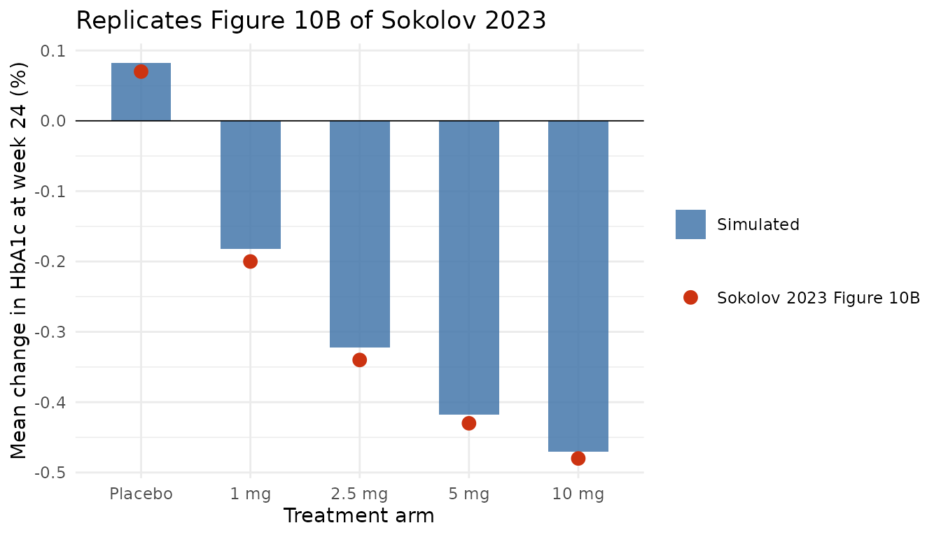
5. Insulin-titration scenario (Figure 10A)
Figure 10A varies the basal insulin dose reduction over 0-90 % and reports that at 10 mg dapagliflozin the 24-week HbA1c reduction is -0.50 % (95% CI -0.553, -0.448) without insulin dose adjustment, rising to -0.42 % (95% CI -0.48, -0.36) when the basal insulin dose is reduced by 50 %.
The “no insulin dose adjustment” arm is the model with
rins pinned at 1, which is obtained exactly by driving
Imax_ins to zero – expit(-30) is below 1e-13
for every individual, whatever the random effect.
sim_noadj <- sim_arm(auc_by_dose[["10 mg"]],
                     params = c(logitimax_ins = -30))
noadj_wk24 <- sim_noadj[sim_noadj$time == 24, ]

cat(sprintf("rins with Imax_ins driven to 0: %.10f\n", max(noadj_wk24$rins)))
#> rins with Imax_ins driven to 0: 1.0000000000
cat(sprintf("10 mg, no basal insulin adjustment: %.3f %% (paper -0.50)\n",
            mean(noadj_wk24$hba1c) - hba1c_bl))
#> 10 mg, no basal insulin adjustment: -0.509 % (paper -0.50)

stopifnot(
  # rins is pinned at 1 for every subject.
  isTRUE(all.equal(max(abs(noadj_wk24$rins - 1)), 0, tolerance = 1e-9)),
  # Paper -0.50 % (95% CI -0.553, -0.448); allow for the cohort draw.
  abs((mean(noadj_wk24$hba1c) - hba1c_bl) - (-0.50)) < 0.10
)
The 50 %-reduction leg of Figure 10A is a property of Equation 2
alone: a basal insulin ratio of 0.5 multiplies the glucose ratio by
0.5^k1. The Abstract states this gives “~5% increase in
glucose exposure”.
k1 <- -0.0674   # Table 3 step 2, sign per the Errata below
glu_increase_50pct <- 0.5^k1 - 1
cat(sprintf("glucose increase for a 50%% basal insulin reduction: %.1f%%\n",
            100 * glu_increase_50pct))
#> glucose increase for a 50% basal insulin reduction: 4.8%

# Propagate through Equation 3 at 10 mg to recover the Figure 10A -0.42 %.
cf_half <- local({
  rins   <- 0.5
  rglu   <- rins^k1 * (1 - 0.15 * 594.3 / (67.4 + 594.3)) + 0.0015 * 24
  # Population mean of k2 (log-normal, median 0.165, omega 0.739 on log scale).
  k2_mean <- 0.165 * exp(0.739^2 / 2)
  rhba1c <- rglu^k2_mean * (1 - 0.0421 * 594.3 / (67.4 + 594.3))
  hba1c_bl * (rhba1c - 1)
})
cat(sprintf("10 mg with a 50%% basal insulin reduction: %.2f %% (paper -0.42)\n",
            cf_half))
#> 10 mg with a 50% basal insulin reduction: -0.42 % (paper -0.42)

stopifnot(
  # Abstract: "~5% increase in glucose exposure".
  glu_increase_50pct > 0.035, glu_increase_50pct < 0.065,
  # Figure 10A: -0.42 % (95% CI -0.48, -0.36).
  cf_half > -0.48, cf_half < -0.36,
  # Withdrawing insulin must WORSEN the HbA1c response relative to no
  # adjustment. This is the assertion that the printed (positive) k1 fails.
  cf_half > (mean(noadj_wk24$hba1c) - hba1c_bl)
)
Exposure-response curves (Figure 7)
Figure 7 plots the predicted change from baseline in basal insulin dose (A), plasma glucose (B) and HbA1c (C) against dapagliflozin exposure over 24 weeks of daily dosing.
auc_grid <- seq(0, 900, by = 10)
curves <- sokolov_closed_form(auc_grid, 24) |>
  transmute(auc,
            `Basal insulin dose` = 100 * (rins - 1),
            `Plasma glucose (CGM)` = 100 * (rglu - 1),
            HbA1c = 100 * (rhba1c - 1)) |>
  tidyr::pivot_longer(-auc, names_to = "endpoint", values_to = "pct_change")
curves$endpoint <- factor(curves$endpoint,
                          levels = c("Basal insulin dose",
                                     "Plasma glucose (CGM)", "HbA1c"))

observed_auc <- data.frame(
  dose = names(auc_by_dose)[-1],
  auc = as.numeric(auc_by_dose[-1])
)

ggplot(curves, aes(x = auc, y = pct_change)) +
  geom_line(linewidth = 0.8, colour = "#4477AA") +
  geom_vline(data = observed_auc, aes(xintercept = auc),
             linetype = "dashed", colour = "grey55", linewidth = 0.3) +
  geom_hline(yintercept = 0, linewidth = 0.3) +
  facet_wrap(~endpoint, scales = "free_y") +
  labs(x = "Dapagliflozin steady-state 24 h AUC (ng*h/mL)",
       y = "Change from baseline at week 24 (%)",
       title = "Replicates Figure 7 of Sokolov 2023",
       subtitle = "Typical-value curves; dashed lines mark the mean AUC at 1, 2.5, 5 and 10 mg") +
  theme_minimal()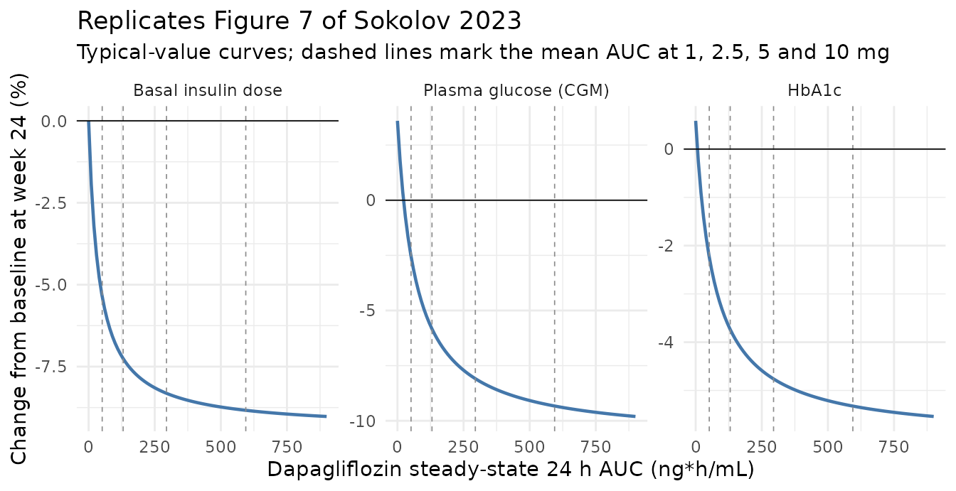
Note that the glucose and HbA1c curves are not monotonically
decreasing at low exposure: the keff * TIME drift term adds
a fixed +3.6 % to the glucose ratio at week 24 regardless of dose, so
the typical-value curve starts above baseline and only crosses zero once
the Imax terms overtake the drift. This reproduces the behaviour the
paper describes for the placebo cohorts.
HbA1c time course
tc <- sim |>
  group_by(arm, time) |>
  summarise(hba1c = mean(hba1c), .groups = "drop")

ggplot(tc, aes(x = time, y = hba1c, colour = arm)) +
  geom_line(linewidth = 0.8) +
  geom_hline(yintercept = hba1c_bl, linetype = "dashed", linewidth = 0.3) +
  labs(x = "Time (weeks)", y = "Mean HbA1c (%)", colour = "Arm",
       title = "Mean HbA1c over the 24-week double-blind period",
       subtitle = "Cohort of 200 subjects per arm; baseline HbA1c 8.48 %") +
  theme_minimal()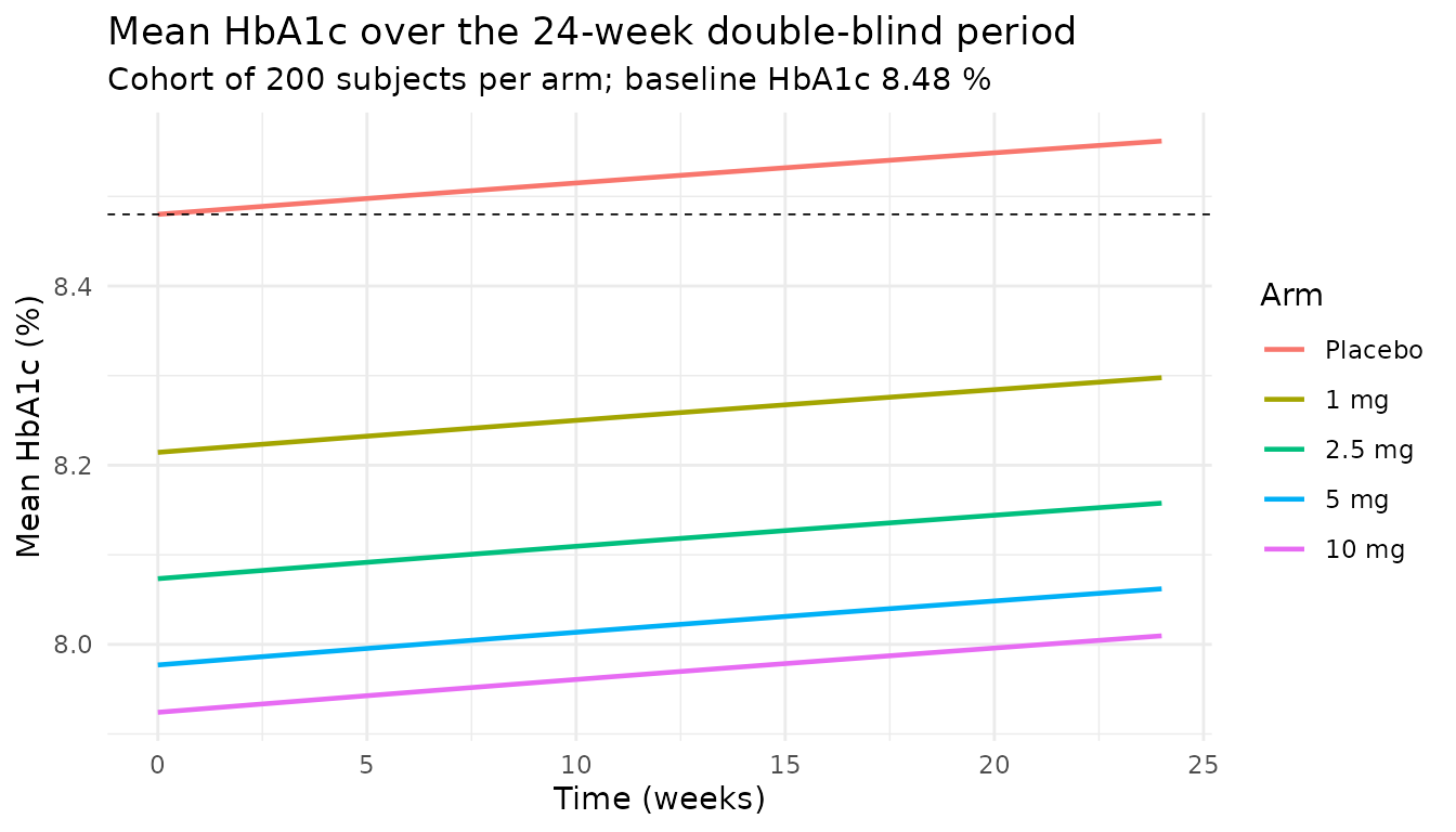
The model has no lag or turnover between glucose and HbA1c – Equation
3 is algebraic – so the HbA1c response is instantaneous at week 0 and
thereafter drifts upward with keff. The paper’s Figure 3
shows most of the observed HbA1c reduction occurring over the first 4
weeks, which this structure approximates as an immediate step; the
source does not fit an HbA1c turnover half-life.
Assumptions and deviations
Sign of k1 (Table 3, step 2). Table 3
prints k1 = 0.0674 with no sign, and Supplementary Equation
2 applies it as the bare exponent (rINS)^k1. Taken
literally, a positive exponent makes plasma glucose
fall when the basal insulin dose is withdrawn, which
contradicts the paper’s own results in four independent places:
- the Abstract and Figure 10A: “a 50% decrease in the basal insulin
dose from pretreatment level, resulting in ~5% increase
in glucose exposure” (
0.5^-0.0674 = 1.048, i.e. +4.8 %; the positive exponent gives -4.6 %); - Figure 10A: the 24-week HbA1c response at 10 mg moves from -0.50 % (no insulin adjustment) to -0.42 % (50 % basal insulin reduction), i.e. withdrawing insulin makes the response worse; the positive exponent predicts -0.58 %, i.e. better;
- Figure 4A: the observed regression of relative change in glucose on relative change in basal insulin dose has slope -0.113;
- physiology, and the sibling M-EASE-1 empagliflozin T1D model
(
Johnston_2021_empagliflozin_MEASE1), whose corresponding insulin-to-glucose power exponent is likewise negative (-0.261).
This file therefore uses ins_glu_eff = -0.0674, i.e. the
printed magnitude with the minus sign restored, and encodes Equation 2
exactly as printed. The stopifnot in section 5 above is the
mechanical guard: it asserts that reducing insulin worsens the HbA1c
response, which is precisely the assertion the printed positive value
fails.
Units of keff (Table 3, step 2). Table
3 labels keff as “mg/dL/week”, but Supplementary Equation 2
adds keff * TIME to rGLU, a unitless
ratio. The term is therefore a fraction of baseline per week:
0.0015 * 24 = +3.6 % at week 24, which matches the
Discussion’s “2%-4% increase in glucose concentration at weeks 12 and
24”. Treating it as mg/dL/week would give a change of 0.036 mg/dL over
24 weeks, which is physically negligible and inconsistent with the
paper’s placebo predictions. The equation governs; the table’s unit
label is taken to be a slip.
Omega scale. Monolix reports omega as
the standard deviation of the random effect. The ini()
block stores variances (1.09^2, 0.003^2,
0.739^2). This reading is corroborated by the fact that it
reproduces Figure 10B at all four doses; treating the values as
variances instead shifts every predicted HbA1c change.
Residual-error scale. All three error models are
applied on the ratio-to-baseline scale, because that is the scale of the
left-hand side of Supplementary Equations 1-3. In particular
a_hba1c = 0.061 is a constant error on rhba1c,
equivalent to about 0.5 % HbA1c at a baseline of 8.48 %, which is a
plausible HbA1c residual; read on the absolute % scale it would imply an
implausibly precise assay.
Upstream population PK. Dapagliflozin AUC is not
modelled here. Table 1 records that AUC values were “taken from a
previously performed population PK analysis (Melin et al., 2022)”, which
is not part of this extraction; the exposure enters as the
AUC_DAPA covariate. The paper publishes the mean AUC at
each dose (Figure 10 caption), which is what this vignette uses, so no
upstream model is needed to reproduce the published results. Users
wanting subject-level exposures can generate them from a dapagliflozin
population PK model such as
modellib("vanderWalt_2013_dapagliflozin").
Bolus insulin and hemoglobin are not in the model.
The paper screened both and excluded them: bolus insulin because it
showed no association with CGM glucose (Figure 4B), and hemoglobin
because the observed change in hemoglobin was not associated with the
change in HbA1c (Figure 5B, all subgroup slope RSEs > 500 %) despite
the ~4 % hemoglobin rise under dapagliflozin. The unexplained
glucose-independent benefit is instead carried by the third Imax term
(imax_hba1c), which the paper estimates contributes about
65 % of the total HbA1c response at 5 and 10 mg.
Absolute versus ratio endpoints. Only HbA1c is
converted to an absolute scale (via the HBA1C baseline
covariate), because Figure 10 reports absolute HbA1c changes. Basal
insulin dose and CGM glucose are left on the ratio scale, matching the
fitted equations; users can rescale them with their own baselines (study
medians: 48-54 units total daily insulin, 170-190 mg/dL mean CGM
glucose).
Cohort size. The paper simulated 500 populations of 500 subjects and reported the mean of means with a 95 % CI reflecting both random effects and parameter uncertainty from the Fisher information matrix. This vignette uses a single cohort of 200 subjects per arm with common random numbers across arms and no parameter-uncertainty sampling, which is sufficient to reproduce the published means but does not reproduce the published CIs.
Monte Carlo tolerances. Per-arm absolute means
depend on which cohort the solver draws; rxSetSeed() fixes
the stream for a given rxode2 build and thread count but not across
them. Measured across three seeds and one, two and four threads, the
placebo-adjusted error stayed below 0.022 % HbA1c while the absolute
per-arm error reached 0.046 %. The assertions above are set at 0.05 %
(placebo-adjusted) and 0.10 % (absolute) accordingly.