Vancomycin MIPD model switch (Tong 2026)
Source:vignettes/articles/Tong_2026_vancomycin.Rmd
Tong_2026_vancomycin.RmdWhat this paper is, and what is extracted from it
Tong 2026 (doi:10.1093/jacamr/dlag016) is not a model-development paper. It is a large quasi-experimental interrupted-time-series study of what happens to clinical outcomes when a model-informed precision dosing (MIPD) service switches the population PK model it doses vancomycin with. Across nineteen US hospital systems and 90 295 patients, two switches were evaluated:
| BMI stratum | Pre-intervention model | Post-intervention model |
|---|---|---|
| BMI < 40 kg/m2 | modified Goti | capped Thomson |
| BMI >= 40 kg/m2 | Carreno | Hughes |
The interrupted-time-series analysis itself is a statistical model and is out of scope for nlmixr2lib. What is in scope is the supplement: its Code section carries the complete NONMEM control stream for all four models exactly as implemented in the InsightRX Nova software, and Tables S1 and S2 tabulate their parameters. Those four streams are the source for the four model files extracted here.
Two points make this paper the primary source for these implementations rather than a redundant restatement of the four upstream publications:
- Three of the four are modified. The “modified Goti” recomputes Cockcroft-Gault creatinine clearance internally and carries a residual-error model that differs from Goti 2018 as published; the “capped Thomson” adds the 150 mL/min creatinine-clearance cap that gives it its name; and the Carreno model has been translated from a non-parametric fit into a parametric one, which required residual-variability assumptions original to this implementation.
-
All four are fixed priors. Tong 2026 estimated no
population parameters. Every value is fixed and used as a prior for MAP
Bayesian estimation of individual parameters, so
fixed()is the faithful encoding throughout.
model_names <- c(
  goti    = "Tong_2026_vancomycin_goti",
  thomson = "Tong_2026_vancomycin_thomson",
  carreno = "Tong_2026_vancomycin_carreno",
  hughes  = "Tong_2026_vancomycin_hughes"
)
mods <- lapply(model_names, function(nm) readModelDb(nm)())
uis  <- lapply(model_names, function(nm) rxode2::rxode(readModelDb(nm)))
names(mods) <- names(uis) <- names(model_names)

tibble::tibble(
  Model      = names(model_names),
  `Model file` = unname(model_names),
  Stratum    = c("BMI < 40 (pre)", "BMI < 40 (post)",
                 "BMI >= 40 (pre)", "BMI >= 40 (post)"),
  Compartments = vapply(uis, function(u) paste(u$state, collapse = ", "), character(1))
) |>
knitr::kable(caption = "The four MIPD models extracted from the Tong 2026 supplement.")| Model | Model file | Stratum | Compartments |
|---|---|---|---|
| goti | Tong_2026_vancomycin_goti | BMI < 40 (pre) | central, peripheral1 |
| thomson | Tong_2026_vancomycin_thomson | BMI < 40 (post) | central, peripheral1 |
| carreno | Tong_2026_vancomycin_carreno | BMI >= 40 (pre) | central, peripheral1 |
| hughes | Tong_2026_vancomycin_hughes | BMI >= 40 (post) | central, peripheral1 |
Population
The cohorts below are the populations these models were applied
to in Tong 2026, not the populations they were estimated from. Each
model file records both: population describes the
application cohort (Table 1), and population$notes records
the upstream development cohort from Table S1 / S2.
pop_tab <- tibble::tribble(
  ~Characteristic,             ~`BMI < 40`,            ~`BMI >= 40`,
  "Patients",                  "87 586",               "2 709",
  "Treatment courses",         "94 991",               "2 964",
  "Samples",                   "192 013",              "6 572",
  "Sex (male/female)",         "39 961 / 55 030",      "1 272 / 1 692",
  "Serum creatinine (mg/dL)",  "0.90 (0.05-25.3)",     "0.95 (0.10-10.9)",
  "Height (cm)",               "170.2 (72.0-256.5)",   "167.6 (93.3-200.7)",
  "Weight (kg)",               "79.0 (20.4-173.8)",    "133.0 (43.8-318.0)",
  "Age (years)",               "65.8 (18.0-90+)",      "60.0 (18.2-90+)"
)
knitr::kable(
  pop_tab,
  caption = paste(
    "Tong 2026 Table 1 (median (min-max) or count). Patients were adults (>= 18 y)",
    "on intravenous vancomycin with at least two doses and one concentration;",
    "haemodialysis patients were excluded."
  )
)| Characteristic | BMI < 40 | BMI >= 40 |
|---|---|---|
| Patients | 87 586 | 2 709 |
| Treatment courses | 94 991 | 2 964 |
| Samples | 192 013 | 6 572 |
| Sex (male/female) | 39 961 / 55 030 | 1 272 / 1 692 |
| Serum creatinine (mg/dL) | 0.90 (0.05-25.3) | 0.95 (0.10-10.9) |
| Height (cm) | 170.2 (72.0-256.5) | 167.6 (93.3-200.7) |
| Weight (kg) | 79.0 (20.4-173.8) | 133.0 (43.8-318.0) |
| Age (years) | 65.8 (18.0-90+) | 60.0 (18.2-90+) |
Development cohorts, from Tables S1 and S2, are much smaller than the application cohorts, and strikingly so for the Carreno model:
tibble::tibble(
  Model = names(model_names),
  `Development patients` = c(1812L, 398L, 12L, 100L),
  `Development samples`  = c(2765L, 1557L, 71L, 276L),
  `Upstream publication` = c("Goti 2018", "Thomson 2009", "Carreno 2017", "Hughes 2024")
) |>
knitr::kable(caption = "Development populations (Tong 2026 Tables S1 and S2).")| Model | Development patients | Development samples | Upstream publication |
|---|---|---|---|
| goti | 1812 | 2765 | Goti 2018 |
| thomson | 398 | 1557 | Thomson 2009 |
| carreno | 12 | 71 | Carreno 2017 |
| hughes | 100 | 276 | Hughes 2024 |
Source trace
Every ini() value in the four model files comes from the
supplement’s Code section (the NONMEM control streams) and is
cross-checked against the printed equations and %CV rows in Tables S1
and S2. The table below records the mapping; the model files carry the
same trace inline, per parameter.
trace <- tibble::tribble(
  ~Model,     ~Quantity,                    ~`Control-stream line`,                                  ~`Table S1 / S2 cross-check`,
  "goti",     "CL 4.5 L/h",                 "$THETA(1) 4.5 FIX",                                     "CL = 4.5 * (CRCLi/120)^0.8",
  "goti",     "Vc 58.4 L",                  "$THETA(2) 58.4 FIX, TVV = THETA(2)*(WT/70)",            "V = 58.4 * WT/70",
  "goti",     "Vp 38.4 L (no WT scaling)",  "$THETA(3) 38.4 FIX, TVV2 = THETA(3)",                   "V2 = 38.4",
  "goti",     "Q 6.5 L/h",                  "$THETA(4) 6.5 FIX",                                     "Q = 6.5",
  "goti",     "CRCL exponent 0.8",          "$THETA(5) 0.8 FIX",                                     "exponent in (CRCLi/120)^0.8",
  "goti",     "Dialysis factors 0.7 / 0.5", "$THETA(6) 0.7 FIX, $THETA(7) 0.5 FIX",                  "not tabulated (structural)",
  "goti",     "CrCL cap 150 mL/min",        "IF(CRCLi.GT.150.0) CRCLi = 150.0",                      "If CRCL > 150, then CRCLi = 150",
  "goti",     "IIV 39.8 / 81.6 / 57.1 %CV", "$OMEGA BLOCK(3) FIX 0.1584, 0.6659, 0.326",             "IIV on CL/V/V2 = 39.8 / 81.6 / 57.1",
  "goti",     "Error 1.42 + 19.7 %",        "$ERROR ADD = 1.42, PROP = 0.197",                       "Additive 1.42, proportional 19.7",
  "thomson",  "CL 2.99 L/h at CrCL 66",     "$THETA(1) 2.99 FIX",                                    "CL = 2.99 * (1 + 0.0154*(CRCLi-66))",
  "thomson",  "Vc 0.675 L/kg",              "$THETA(2) 0.675 FIX, TVV = THETA(2)*WT",                "V = 0.675 * WT",
  "thomson",  "CRCL slope 0.0154",          "$THETA(3) 0.0154 FIX",                                  "slope in (1 + 0.0154*(CRCLi-66))",
  "thomson",  "Q 2.28 L/h",                 "$THETA(4) 2.28 FIX",                                    "Q = 2.28",
  "thomson",  "Vp 0.732 L/kg",              "$THETA(5) 0.732 FIX, TVV2 = THETA(5)*WT",               "V2 = 0.732 * WT",
  "thomson",  "CrCL cap 150 mL/min",        "IF(EGFR.GT.CRCLCAP) CRCLcapped = CRCLCAP",              "If CRCL > 150, then CRCLi = 150",
  "thomson",  "IIV 27 / 15 %CV + cov",      "$OMEGA BLOCK(2) FIX 0.0729 / 0.01 0.0225",              "IIV on CL/V = 27 / 15",
  "thomson",  "IIV Q 49, V2 130 %CV",       "$OMEGA 0.2401 FIX; $OMEGA 1.69 FIX",                    "IIV on Q/V2 = 49 / 130",
  "thomson",  "Error 1.6 + 15 %",           "$ERROR ADD = 1.6, PROP = 0.15",                         "Additive 1.6, proportional 15",
  "carreno",  "CL intercept 0.18 L/h",      "$THETA(5) 0.18 FIX (TVSCLINTER)",                       "CL = 0.18 + 0.036 * CRCL",
  "carreno",  "CL slope 0.036",             "$THETA(2) 0.036 FIX (TVSCLSLOPE)",                      "CL = 0.18 + 0.036 * CRCL",
  "carreno",  "Vc 25.76 L",                 "$THETA(1) 25.76 FIX",                                   "V = 25.76",
  "carreno",  "k12 2.29 /h, k21 1.44 /h",   "$THETA(3) 2.29 FIX, $THETA(4) 1.44 FIX",                "Q = 2.29*25.76; V2 = Q/1.44",
  "carreno",  "IIV 45.3/55.6/105.6/120.1/23.9", "$OMEGA BLOCK(5) 0.20559 ... 0.057068",              "IIV rows of Table S2",
  "carreno",  "Error 0.1 + 10 %",           "$ERROR ADD = 0.1, PROP = 0.1",                          "Additive 0.1, proportional 10",
  "hughes",   "CL 5.0627 L/h at CrCL 100",  "$THETA(1) 5.0627",                                      "CL = 5.06 * (CRCL/100)^0.8509",
  "hughes",   "Vc 64.339 L at FFM 70",      "$THETA(2) 64.339",                                      "V = 64.339 * FFM/70",
  "hughes",   "Q 6.2402 L/h",               "$THETA(3) 6.2402",                                      "Q = 6.2402",
  "hughes",   "Vp 59.019 L at FFM 70",      "$THETA(4) 59.019",                                      "V2 = 59.019 * FFM/70",
  "hughes",   "FFM exponent 1 (fixed)",     "$THETA(7) 1 FIX  ; allo V1/V2",                         "linear FFM/70 in both volumes",
  "hughes",   "CRCL exponent 0.8509",       "$THETA(8) 0.8509",                                      "exponent in (CRCL/100)^0.8509",
  "hughes",   "IIV 21.8 / 18.0 / 79.7 %CV", "$OMEGA BLOCK(3) 0.0473154 ... 0.634656",                "IIV on CL/V/V2 = 21.8 / 18.0 / 79.7",
  "hughes",   "Error 0.001 + 13.72 %",      "$THETA(6) 0.001, $THETA(5) 0.1372",                     "Additive '-', proportional 13.3 (see Errata)"
)
knitr::kable(
  trace,
  caption = paste(
    "Source trace. 'Control-stream line' refers to the Tong 2026 Supplementary",
    "data, Code section; Tables S1 (BMI < 40) and S2 (BMI >= 40) provide the",
    "independent cross-check."
  )
)| Model | Quantity | Control-stream line | Table S1 / S2 cross-check |
|---|---|---|---|
| goti | CL 4.5 L/h | THETA(2) 58.4 FIX, TVV = THETA(2)*(WT/70) | V = 58.4 * WT/70 |
| goti | Vp 38.4 L (no WT scaling) | THETA(4) 6.5 FIX | Q = 6.5 |
| goti | CRCL exponent 0.8 | THETA(6) 0.7 FIX, OMEGA BLOCK(3) FIX 0.1584, 0.6659, 0.326 | IIV on CL/V/V2 = 39.8 / 81.6 / 57.1 |
| goti | Error 1.42 + 19.7 % | THETA(1) 2.99 FIX | CL = 2.99 * (1 + 0.0154*(CRCLi-66)) |
| thomson | Vc 0.675 L/kg | THETA(3) 0.0154 FIX | slope in (1 + 0.0154*(CRCLi-66)) |
| thomson | Q 2.28 L/h | THETA(5) 0.732 FIX, TVV2 = THETA(5)*WT | V2 = 0.732 * WT |
| thomson | CrCL cap 150 mL/min | IF(EGFR.GT.CRCLCAP) CRCLcapped = CRCLCAP | If CRCL > 150, then CRCLi = 150 |
| thomson | IIV 27 / 15 %CV + cov | OMEGA 0.2401 FIX; ERROR ADD = 1.6, PROP = 0.15 | Additive 1.6, proportional 15 |
| carreno | CL intercept 0.18 L/h | THETA(2) 0.036 FIX (TVSCLSLOPE) | CL = 0.18 + 0.036 * CRCL |
| carreno | Vc 25.76 L | THETA(3) 2.29 FIX, OMEGA BLOCK(5) 0.20559 … 0.057068 | IIV rows of Table S2 |
| carreno | Error 0.1 + 10 % | THETA(1) 5.0627 | CL = 5.06 * (CRCL/100)^0.8509 |
| hughes | Vc 64.339 L at FFM 70 | THETA(3) 6.2402 | Q = 6.2402 |
| hughes | Vp 59.019 L at FFM 70 | THETA(7) 1 FIX ; allo V1/V2 | linear FFM/70 in both volumes |
| hughes | CRCL exponent 0.8509 | OMEGA BLOCK(3) 0.0473154 … 0.634656 | IIV on CL/V/V2 = 21.8 / 18.0 / 79.7 |
| hughes | Error 0.001 + 13.72 % | $THETA(6) 0.001, $THETA(5) 0.1372 | Additive ‘-’, proportional 13.3 (see Errata) |
A structural detail worth recording, because it is easy to get wrong:
both control streams that compute Cockcroft-Gault internally write the
sex factor as 0.85**(1-SEX), i.e. SEX = 1 denotes
male. The Hughes stream confirms this independently, because
its IF(SEX.EQ.0) branch selects the female
Janmahasatian fat-free-mass coefficients. The model files therefore
store the canonical SEXF (1 = female) and write the factor
as 0.85^SEXF.
Check 1: the models reproduce the printed Table S1 / S2 equations
The strongest available source-trace check is deterministic: for a reference patient, solve each model and confirm the individual parameters equal the equations printed in Tables S1 and S2. No simulation noise, no seed dependence.
solve_typical <- function(mod, cov) {
  ev <- rxode2::et(amt = 1000, cmt = "central", dur = 1) |>
    rxode2::et(c(0.5, 2), cmt = "central")
  as.data.frame(rxode2::rxSolve(rxode2::zeroRe(mod), ev, params = cov,
                                returnType = "data.frame"))
}

# Reference patient for the BMI < 40 models: 70 kg, 40 y, male, SCr 0.9 mg/dL.
cg_ref  <- (140 - 40) * 70 * 0.85^0 / (72 * 0.9)
s_goti  <- solve_typical(mods$goti,
  data.frame(AGE = 40, WT = 70, SEXF = 0, CREAT = 0.9, RRT_HEMODIAL_STATUS = 0))
#> ℹ omega/sigma items treated as zero: 'etalcl', 'etalvc', 'etalvp'
s_thom  <- solve_typical(mods$thomson, data.frame(WT = 70, CRCL = 100))
#> ℹ omega/sigma items treated as zero: 'etalcl', 'etalvc', 'etalq', 'etalvp'

# Reference patient for the BMI >= 40 models: 133 kg, 167.6 cm, 60 y, female.
bmi_ref  <- 133 / (167.6 / 100)^2
ffm_ref  <- 9270 * 133 / (8780 + 244 * bmi_ref)
crcl_ref <- (140 - 60) * ffm_ref * 0.85 / (72 * 0.95)
s_carr   <- solve_typical(mods$carreno, data.frame(CRCL = 100))
#> ℹ omega/sigma items treated as zero: 'etalvc', 'etalcl_renal', 'etalk12', 'etalk21', 'etalcl_nonren'
s_hugh   <- solve_typical(mods$hughes,
  data.frame(WT = 133, HT = 167.6, AGE = 60, SEXF = 1, CREAT = 0.95))
#> ℹ omega/sigma items treated as zero: 'etalcl', 'etalvc', 'etalvp'

tv <- tibble::tribble(
  ~Model, ~Parameter, ~Simulated, ~`Table S1 / S2 equation`, ~Expected,
  "goti",    "CL (L/h)", s_goti$cl[1], "4.5 * (CRCLi/120)^0.8",   4.5 * (cg_ref / 120)^0.8,
  "goti",    "Vc (L)",   s_goti$vc[1], "58.4 * WT/70",            58.4 * 70 / 70,
  "goti",    "Vp (L)",   s_goti$vp[1], "38.4",                    38.4,
  "goti",    "Q (L/h)",  s_goti$q[1],  "6.5",                     6.5,
  "thomson", "CL (L/h)", s_thom$cl[1], "2.99 * (1 + 0.0154*(CRCL-66))", 2.99 * (1 + 0.0154 * (100 - 66)),
  "thomson", "Vc (L)",   s_thom$vc[1], "0.675 * WT",              0.675 * 70,
  "thomson", "Vp (L)",   s_thom$vp[1], "0.732 * WT",              0.732 * 70,
  "thomson", "Q (L/h)",  s_thom$q[1],  "2.28",                    2.28,
  "carreno", "CL (L/h)", s_carr$cl[1], "0.18 + 0.036 * CRCL",     0.18 + 0.036 * 100,
  "carreno", "Vc (L)",   s_carr$vc[1], "25.76",                   25.76,
  "carreno", "Q (L/h)",  s_carr$q[1],  "k12 * V = 2.29 * 25.76",  2.29 * 25.76,
  "carreno", "Vp (L)",   s_carr$vp[1], "Q / k21 = Q / 1.44",      2.29 * 25.76 / 1.44,
  "hughes",  "CL (L/h)", s_hugh$cl[1], "5.0627 * (CRCL/100)^0.8509", 5.0627 * (crcl_ref / 100)^0.8509,
  "hughes",  "Vc (L)",   s_hugh$vc[1], "64.339 * FFM/70",         64.339 * ffm_ref / 70,
  "hughes",  "Vp (L)",   s_hugh$vp[1], "59.019 * FFM/70",         59.019 * ffm_ref / 70,
  "hughes",  "Q (L/h)",  s_hugh$q[1],  "6.2402",                  6.2402
) |>
  mutate(`% diff` = 100 * (Simulated - Expected) / Expected)

tv |>
  mutate(across(c(Simulated, Expected), ~ round(.x, 4)),
         `% diff` = signif(`% diff`, 3)) |>
  knitr::kable(caption = paste(
    "Check 1. Individual parameters solved from each model file against the",
    "equation printed in Tong 2026 Table S1 / S2. The reference patients are",
    sprintf("70 kg / 40 y / male / SCr 0.9 (Cockcroft-Gault %.1f mL/min) and", cg_ref),
    sprintf("133 kg / 167.6 cm / 60 y / female (FFM %.1f kg, CrCL %.1f mL/min).",
            ffm_ref, crcl_ref)
))| Model | Parameter | Simulated | Table S1 / S2 equation | Expected | % diff |
|---|---|---|---|---|---|
| goti | CL (L/h) | 4.1370 | 4.5 * (CRCLi/120)^0.8 | 4.1370 | 0 |
| goti | Vc (L) | 58.4000 | 58.4 * WT/70 | 58.4000 | 0 |
| goti | Vp (L) | 38.4000 | 38.4 | 38.4000 | 0 |
| goti | Q (L/h) | 6.5000 | 6.5 | 6.5000 | 0 |
| thomson | CL (L/h) | 4.5556 | 2.99 * (1 + 0.0154*(CRCL-66)) | 4.5556 | 0 |
| thomson | Vc (L) | 47.2500 | 0.675 * WT | 47.2500 | 0 |
| thomson | Vp (L) | 51.2400 | 0.732 * WT | 51.2400 | 0 |
| thomson | Q (L/h) | 2.2800 | 2.28 | 2.2800 | 0 |
| carreno | CL (L/h) | 3.7800 | 0.18 + 0.036 * CRCL | 3.7800 | 0 |
| carreno | Vc (L) | 25.7600 | 25.76 | 25.7600 | 0 |
| carreno | Q (L/h) | 58.9904 | k12 * V = 2.29 * 25.76 | 58.9904 | 0 |
| carreno | Vp (L) | 40.9656 | Q / k21 = Q / 1.44 | 40.9656 | 0 |
| hughes | CL (L/h) | 3.2911 | 5.0627 * (CRCL/100)^0.8509 | 3.2911 | 0 |
| hughes | Vc (L) | 55.7323 | 64.339 * FFM/70 | 55.7323 | 0 |
| hughes | Vp (L) | 51.1240 | 59.019 * FFM/70 | 51.1240 | 0 |
| hughes | Q (L/h) | 6.2402 | 6.2402 | 6.2402 | 0 |
# The printed equations are exact algebra, so this must match to solver precision.
stopifnot(max(abs(tv$`% diff`)) < 1e-6)
That every one of the sixteen rows matches to solver precision is the check that the transcription of the four control streams is correct: it exercises the Cockcroft-Gault derivation, the Janmahasatian fat-free-mass branch, the sex polarity conversion, the linear-versus-power renal terms, the per-kg versus per-70-kg volume conventions, and the Carreno k12 / k21 to Q / Vp derivation.
Check 1b: the closed-form and ODE solvers agree
rxSolve() with useLinCmt = TRUE rewrites a
recognisably linear two-compartment system into a closed form. When such
a model is written straight from stored micro-constants, that rewrite
can silently drop peripheral1 and solve a
one-compartment model instead – with total AUC unchanged, so an
exposure check will not catch it. The readout that moves is the terminal
half-life.
All four models are therefore written so the peripheral transfer is
expressed as q and vp, and the equivalence is
asserted mechanically rather than assumed. This is a regression gate: an
earlier draft of the Carreno file stored k12 and
k21 directly and collapsed to 5.22 h against a true 13.82
h.
beta_half_life <- function(kel, k12, k21) {
  b <- kel + k12 + k21
  log(2) / ((b - sqrt(b^2 - 4 * kel * k21)) / 2)
}

# Sampling runs to 200 h and the slope is taken over 100-200 h. The capped
# Thomson model has a small Q against a large peripheral volume, so its
# distribution phase is still resolving at 72 h; by 100 h all four models are in
# the true terminal phase and the fitted slope is the beta root to 4 figures.
lincmt_ev <- as.data.frame(
  rxode2::et(amt = 1500, cmt = "central", dur = 1.5) |>
    rxode2::et(seq(0, 200, by = 0.5), cmt = "central")
)
lincmt_ev$id <- 1L

lincmt_cov <- list(
  goti    = list(WT = 79, AGE = 65, SEXF = 1, CREAT = 0.9,
                 RRT_HEMODIAL_STATUS = 0),
  thomson = list(WT = 79, CRCL = 90),
  carreno = list(CRCL = 90),
  hughes  = list(WT = 133, HT = 167.6, AGE = 60, SEXF = 1, CREAT = 0.95)
)

lincmt_chk <- dplyr::bind_rows(lapply(names(lincmt_cov), function(nm) {
  ev <- lincmt_ev
  for (cn in names(lincmt_cov[[nm]])) ev[[cn]] <- lincmt_cov[[nm]][[cn]]
  hl <- vapply(c(TRUE, FALSE), function(lin) {
    s <- as.data.frame(rxode2::rxSolve(rxode2::zeroRe(mods[[nm]]), ev,
                                       useLinCmt = lin, returnType = "data.frame"))
    # Keep Cc >= 1e-6 of Cmax: below that the ODE tail is solver noise.
    s <- s[s$time >= 100 & s$Cc >= 1e-6 * max(s$Cc), ]
    -log(2) / stats::coef(stats::lm(log(Cc) ~ time, data = s))[["time"]]
  }, numeric(1))
  s <- as.data.frame(rxode2::rxSolve(rxode2::zeroRe(mods[[nm]]), ev,
                                     returnType = "data.frame"))
  tibble::tibble(
    Model            = nm,
    `t1/2 closed form (h)` = hl[[1]],
    `t1/2 ODE (h)`         = hl[[2]],
    `t1/2 analytic (h)`    = beta_half_life(s$kel[1], s$k12[1], s$k21[1]),
    `t1/2 if collapsed (h)` = log(2) / s$kel[1]
  )
}))
#> ℹ omega/sigma items treated as zero: 'etalcl', 'etalvc', 'etalvp'
#> ℹ omega/sigma items treated as zero: 'etalcl', 'etalvc', 'etalvp'
#> ℹ omega/sigma items treated as zero: 'etalcl', 'etalvc', 'etalvp'
#> ℹ omega/sigma items treated as zero: 'etalcl', 'etalvc', 'etalq', 'etalvp'
#> ℹ omega/sigma items treated as zero: 'etalcl', 'etalvc', 'etalq', 'etalvp'
#> ℹ omega/sigma items treated as zero: 'etalcl', 'etalvc', 'etalq', 'etalvp'
#> ℹ omega/sigma items treated as zero: 'etalvc', 'etalcl_renal', 'etalk12', 'etalk21', 'etalcl_nonren'
#> ℹ omega/sigma items treated as zero: 'etalvc', 'etalcl_renal', 'etalk12', 'etalk21', 'etalcl_nonren'
#> ℹ omega/sigma items treated as zero: 'etalvc', 'etalcl_renal', 'etalk12', 'etalk21', 'etalcl_nonren'
#> ℹ omega/sigma items treated as zero: 'etalcl', 'etalvc', 'etalvp'
#> ℹ omega/sigma items treated as zero: 'etalcl', 'etalvc', 'etalvp'
#> ℹ omega/sigma items treated as zero: 'etalcl', 'etalvc', 'etalvp'

lincmt_chk |>
  dplyr::mutate(dplyr::across(where(is.numeric), ~ round(.x, 3))) |>
  knitr::kable(caption = paste(
    "Check 1b. Terminal half-life recovered from the closed-form solver, from",
    "the ODE solver, and from the analytic beta root of the two-compartment",
    "system. The last column is what a collapsed one-compartment rewrite would",
    "return; it is roughly half the correct value in every case, which is what",
    "makes this gate sensitive."
))| Model | t1/2 closed form (h) | t1/2 ODE (h) | t1/2 analytic (h) | t1/2 if collapsed (h) |
|---|---|---|---|---|
| goti | 24.429 | 24.429 | 24.429 | 14.371 |
| thomson | 31.329 | 31.329 | 31.330 | 9.026 |
| carreno | 13.823 | 13.823 | 13.823 | 5.221 |
| hughes | 25.578 | 25.578 | 25.578 | 11.738 |
# All three must agree: the two solvers exactly, and both against the analytic
# beta root to log-linear regression precision.
stopifnot(
  max(abs(lincmt_chk$`t1/2 closed form (h)` /
          lincmt_chk$`t1/2 ODE (h)` - 1)) < 1e-6,
  max(abs(lincmt_chk$`t1/2 ODE (h)` /
          lincmt_chk$`t1/2 analytic (h)` - 1)) < 1e-3,
  # The gate would be vacuous if the collapsed value were close to the correct
  # one; assert that it is not, so a future regression cannot slip through.
  all(lincmt_chk$`t1/2 if collapsed (h)` <
        0.75 * lincmt_chk$`t1/2 analytic (h)`)
)
Check 2: steady-state exposure equals Dose / CL
For any linear model, the AUC over one dosing interval at steady state equals Dose / CL exactly. This is independent of the number of compartments and of the distribution parameters, so it is a clean test that the clearance parameterisation and the dose-to-concentration unit chain are right in all four models. Dosing runs long enough for the slowest subject in the cohort to reach steady state (120 doses at q12h, about 60 days; the slowest subjects here have terminal half-lives near 70 h).
rxode2::rxSetSeed(20260828)
set.seed(20260828)

n_per_arm <- 100  # well within the 200-per-arm cap
tau       <- 12
n_dose    <- 120
ss_start  <- (n_dose - 1) * tau
ss_end    <- n_dose * tau

# BMI < 40 cohort, marginals from Tong 2026 Table 1.
coh_lo <- tibble::tibble(
  id    = seq_len(n_per_arm),
  WT    = pmin(pmax(exp(rnorm(n_per_arm, log(79), 0.26)), 20.4), 173.8),
  AGE   = pmin(pmax(rnorm(n_per_arm, 65.8, 15), 18), 90),
  SEXF  = rbinom(n_per_arm, 1, 0.579),
  CREAT = pmin(pmax(exp(rnorm(n_per_arm, log(0.90), 0.45)), 0.05), 25.3),
  RRT_HEMODIAL_STATUS = 0
) |>
  mutate(
    # The MIPD pipeline computes capped Cockcroft-Gault once and feeds it to
    # whichever model needs CRCL as a data item (the Thomson variant).
    CRCL = pmin((140 - AGE) * WT * 0.85^SEXF / (72 * CREAT), 150),
    HT   = 170.2,
    dose = pmin(pmax(round(15 * WT / 250) * 250, 500), 2000)
  )

# BMI >= 40 cohort, marginals from Tong 2026 Table 1.
coh_hi <- tibble::tibble(
  id    = seq_len(n_per_arm),
  WT    = pmin(pmax(exp(rnorm(n_per_arm, log(133), 0.24)), 43.8), 318.0),
  HT    = pmin(pmax(rnorm(n_per_arm, 167.6, 11), 93.3), 200.7),
  AGE   = pmin(pmax(rnorm(n_per_arm, 60.0, 15), 18), 90),
  SEXF  = rbinom(n_per_arm, 1, 0.571),
  CREAT = pmin(pmax(exp(rnorm(n_per_arm, log(0.95), 0.45)), 0.10), 10.9),
  RRT_HEMODIAL_STATUS = 0
) |>
  mutate(
    CRCL = pmin((140 - AGE) * WT * 0.85^SEXF / (72 * CREAT), 150),
    dose = pmin(pmax(round(15 * WT / 250) * 250, 500), 2500)
  )

tibble::tibble(
  Cohort = c("BMI < 40", "BMI >= 40"),
  `WT median` = c(median(coh_lo$WT), median(coh_hi$WT)),
  `AGE median` = c(median(coh_lo$AGE), median(coh_hi$AGE)),
  `CREAT median` = c(median(coh_lo$CREAT), median(coh_hi$CREAT)),
  `CRCL median` = c(median(coh_lo$CRCL), median(coh_hi$CRCL)),
  `Dose median (mg)` = c(median(coh_lo$dose), median(coh_hi$dose))
) |>
  mutate(across(where(is.numeric), ~ round(.x, 1))) |>
  knitr::kable(caption = paste(
    "Virtual cohorts, 100 subjects per arm. Marginal distributions are matched",
    "to the Tong 2026 Table 1 medians and truncated to its observed ranges;",
    "the joint distribution is not recoverable from the paper (see Assumptions)."
))| Cohort | WT median | AGE median | CREAT median | CRCL median | Dose median (mg) |
|---|---|---|---|---|---|
| BMI < 40 | 78.3 | 64.1 | 1.1 | 68.3 | 1250 |
| BMI >= 40 | 137.9 | 60.1 | 1.0 | 137.1 | 2000 |
build_events <- function(coh) {
  ev <- lapply(seq_len(nrow(coh)), function(i) {
    e <- as.data.frame(
      rxode2::et(amt = coh$dose[[i]], cmt = "central", dur = 1,
                 ii = tau, addl = n_dose - 1) |>
        rxode2::et(seq(ss_start, ss_end, by = 0.1), cmt = "central")
    )
    e$id <- coh$id[[i]]
    e
  })
  ev <- dplyr::bind_rows(ev)
  # Covariates are attached to the materialised data frame, never to the rxEt
  # object (rxode2 silently drops assignments made to an rxEt).
  ev <- dplyr::left_join(
    ev,
    dplyr::select(coh, id, WT, HT, AGE, SEXF, CREAT, RRT_HEMODIAL_STATUS, CRCL),
    by = "id"
  )
  dplyr::arrange(ev, id, time, dplyr::desc(evid))
}

ev_lo <- build_events(coh_lo)
ev_hi <- build_events(coh_hi)

solve_apriori <- function(mod, ev) {
  as.data.frame(rxode2::rxSolve(rxode2::zeroRe(mod), ev, returnType = "data.frame"))
}

sims <- list(
  goti    = solve_apriori(mods$goti,    ev_lo),
  thomson = solve_apriori(mods$thomson, ev_lo),
  carreno = solve_apriori(mods$carreno, ev_hi),
  hughes  = solve_apriori(mods$hughes,  ev_hi)
)
#> ℹ omega/sigma items treated as zero: 'etalcl', 'etalvc', 'etalvp'
#> Warning: multi-subject simulation without without 'omega'
#> ℹ omega/sigma items treated as zero: 'etalcl', 'etalvc', 'etalq', 'etalvp'
#> Warning: multi-subject simulation without without 'omega'
#> ℹ omega/sigma items treated as zero: 'etalvc', 'etalcl_renal', 'etalk12', 'etalk21', 'etalcl_nonren'
#> Warning: multi-subject simulation without without 'omega'
#> ℹ omega/sigma items treated as zero: 'etalcl', 'etalvc', 'etalvp'
#> Warning: multi-subject simulation without without 'omega'
stopifnot(vapply(sims, function(s) all(!is.na(s$Cc)), logical(1)))
stopifnot(vapply(sims, function(s) all(s$Cc >= 0), logical(1)))
These are a priori predictions in the sense the paper uses:
population-level predictions from the patient’s covariates with no
concentration data and hence no individual random effects, which is what
drives the initial dosing decision. zeroRe() supplies
exactly that, and makes the result deterministic rather than
seed-dependent.
# ID offsets keep subjects disjoint across the four model arms so PKNCA never
# pools two different subjects under one id.
id_offset <- c(goti = 0L, thomson = 1000L, carreno = 2000L, hughes = 3000L)

conc_all <- dplyr::bind_rows(lapply(names(sims), function(nm) {
  sims[[nm]] |>
    dplyr::filter(!is.na(Cc)) |>
    dplyr::transmute(id = id + id_offset[[nm]], time = time, Cc = Cc,
                     treatment = nm)
}))

dose_all <- dplyr::bind_rows(lapply(names(sims), function(nm) {
  coh <- if (nm %in% c("goti", "thomson")) coh_lo else coh_hi
  # PKNCA needs a dose record inside the steady-state interval.
  tibble::tibble(id = coh$id + id_offset[[nm]], time = ss_start,
                 amt = coh$dose, treatment = nm)
}))

conc_obj <- PKNCA::PKNCAconc(as.data.frame(conc_all), Cc ~ time | treatment + id,
                             concu = "mg/L", timeu = "h")
dose_obj <- PKNCA::PKNCAdose(as.data.frame(dose_all), amt ~ time | treatment + id,
                             doseu = "mg")

intervals_ss <- data.frame(
  start = ss_start, end = ss_end,
  cmax = TRUE, tmax = TRUE, cmin = TRUE,
  cav = TRUE, auclast = TRUE
)
# PKNCA's `ctrough` is deliberately not requested: it is defined at a dosing
# time, and this interval ends one dosing interval after the last dose, so it
# would be NA for every subject. `cmin` -- the minimum over the interval -- is
# the trough at steady state, and is checked against the simulated profile
# directly below.

nca_ss <- PKNCA::pk.nca(PKNCA::PKNCAdata(conc_obj, dose_obj,
                                         intervals = intervals_ss))
nca_tbl <- as.data.frame(nca_ss$result)
auc_ss <- nca_tbl |>
  dplyr::filter(PPTESTCD == "auclast") |>
  dplyr::transmute(id, treatment, auc_tau = PPORRES)

cl_ss <- dplyr::bind_rows(lapply(names(sims), function(nm) {
  sims[[nm]] |>
    dplyr::group_by(id) |>
    dplyr::summarise(cl = dplyr::first(cl), .groups = "drop") |>
    dplyr::mutate(id = id + id_offset[[nm]], treatment = nm)
}))

dose_lookup <- dose_all |> dplyr::select(id, treatment, amt)

ss_chk <- auc_ss |>
  dplyr::inner_join(cl_ss, by = c("id", "treatment")) |>
  dplyr::inner_join(dose_lookup, by = c("id", "treatment")) |>
  dplyr::mutate(pred = amt / cl,
                pct_diff = 100 * (auc_tau - pred) / pred)

ss_chk |>
  dplyr::group_by(treatment) |>
  dplyr::summarise(
    n = dplyr::n(),
    `median AUCtau (mg*h/L)` = round(median(auc_tau), 1),
    `median Dose/CL (mg*h/L)` = round(median(pred), 1),
    `max |% diff|` = signif(max(abs(pct_diff)), 3),
    .groups = "drop"
  ) |>
  knitr::kable(caption = paste(
    "Check 2. PKNCA AUC over the steady-state dosing interval against the exact",
    "linear-system identity Dose / CL, for every subject in every arm."
))| treatment | n | median AUCtau (mg*h/L) | median Dose/CL (mg*h/L) | max |% diff| |
|---|---|---|---|---|
| carreno | 100 | 448.0 | 448.0 | 0.00230 |
| goti | 100 | 406.7 | 406.7 | 0.00140 |
| hughes | 100 | 576.2 | 576.2 | 0.00157 |
| thomson | 100 | 372.7 | 372.7 | 0.00331 |
Check 3: the two BMI < 40 clearance models cross over near 50 mL/min
The paper’s central pharmacological finding is that the modified Goti model estimates AUC higher than the capped Thomson model, and that this is what shifted target attainment when sites switched. The mechanism is entirely in the two clearance submodels: Goti uses a power function of creatinine clearance normalised at 120 mL/min, Thomson a linear function centred at 66 mL/min. Because one is concave and the other linear, they cross.
sweep <- tibble::tibble(CRCL = seq(20, 150, by = 1)) |>
  mutate(
    `modified Goti`  = 4.5 * (CRCL / 120)^0.8,
    `capped Thomson` = 2.99 * (1 + 0.0154 * (CRCL - 66))
  )

crossover <- sweep$CRCL[which.min(abs(sweep$`modified Goti` - sweep$`capped Thomson`))]

sweep |>
  tidyr::pivot_longer(-CRCL, names_to = "Model", values_to = "CL") |>
  ggplot(aes(CRCL, CL, colour = Model)) +
  geom_line(linewidth = 0.9) +
  geom_vline(xintercept = crossover, linetype = "dashed", colour = "grey40") +
  annotate("text", x = crossover + 3, y = max(sweep$`capped Thomson`) * 0.35,
           label = paste0("crossover ~", crossover, " mL/min"),
           hjust = 0, size = 3.2, colour = "grey30") +
  labs(x = "Creatinine clearance (mL/min)", y = "A priori CL (L/h)",
       colour = NULL) +
  theme_bw() +
  theme(legend.position = "top")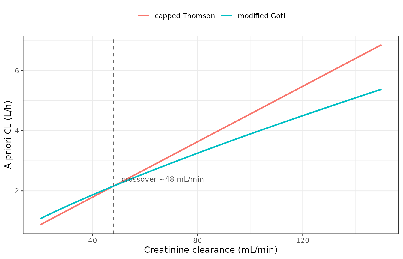
A priori clearance under the two BMI < 40 models as a function of creatinine clearance. The models cross near 49 mL/min; above it Goti predicts lower clearance and therefore higher AUC, which is the direction Tong 2026 reports.
# Structural consequences of the two functional forms.
stopifnot(
  crossover > 40, crossover < 60,
  # Above the crossover Thomson clears faster, so Goti gives the higher AUC.
  with(sweep, all((`capped Thomson` > `modified Goti`)[CRCL > crossover + 5])),
  # Below it the ordering reverses.
  with(sweep, all((`capped Thomson` < `modified Goti`)[CRCL < crossover - 5]))
)
The population median creatinine clearance implied by Table 1 (age 65.8 y, 79 kg, 58% female, SCr 0.90 mg/dL) is about 77 mL/min, comfortably above the crossover. So most patients sit in the region where Goti predicts the higher AUC, and a low-renal-function minority sits in the region where the ordering reverses.
Check 4: a priori AUC agreement, replicating Figure S4
Tong 2026 reports a Bland-Altman comparison of a priori AUC between the two BMI < 40 models: the modified Goti model estimated AUCs +17.5 mg*h/L higher than the capped Thomson model on average, one patient in 13 (7.7%) differed by more than 20%, and the discordance was “driven primarily by the Goti model estimating higher AUCs” (5.9% of patients).
auc24 <- auc_ss |>
  dplyr::filter(treatment %in% c("goti", "thomson")) |>
  dplyr::mutate(id = id - id_offset[treatment],
                auc24 = 2 * auc_tau) |>
  dplyr::select(id, treatment, auc24) |>
  tidyr::pivot_wider(names_from = treatment, values_from = auc24)

ba <- auc24 |>
  dplyr::mutate(
    mean_auc = (goti + thomson) / 2,
    diff_auc = goti - thomson,
    pct_diff = 100 * diff_auc / mean_auc
  )

ggplot(ba, aes(mean_auc, diff_auc)) +
  geom_hline(yintercept = 0, colour = "grey70") +
  geom_hline(yintercept = mean(ba$diff_auc), linetype = "dashed",
             colour = "steelblue") +
  geom_line(aes(y = 0.2 * mean_auc), linetype = "dotted", colour = "grey40") +
  geom_line(aes(y = -0.2 * mean_auc), linetype = "dotted", colour = "grey40") +
  geom_point(alpha = 0.6, size = 1.6) +
  labs(x = "Mean of the two a priori AUC24 estimates (mg*h/L)",
       y = "Goti - Thomson (mg*h/L)") +
  theme_bw()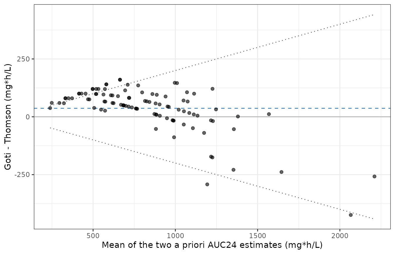
Replicates Figure S4 of Tong 2026. Bland-Altman comparison of a priori steady-state AUC24 between the modified Goti and capped Thomson models over the virtual BMI < 40 cohort. Dashed line is the mean difference; dotted lines are the +/- 20% relative-difference boundaries.
ba_stats <- tibble::tribble(
  ~Metric,                                    ~Published, ~Simulated,
  "Mean difference, Goti - Thomson (mg*h/L)", "+17.5",    sprintf("%+.1f", mean(ba$diff_auc)),
  "Patients differing by > 20%",              "7.7%",     sprintf("%.1f%%", 100 * mean(abs(ba$pct_diff) > 20)),
  "Goti higher by > 20%",                     "5.9%",     sprintf("%.1f%%", 100 * mean(ba$pct_diff > 20)),
  "Thomson higher by > 20%",                  "1.8%",     sprintf("%.1f%%", 100 * mean(ba$pct_diff < -20))
)
knitr::kable(ba_stats, caption = paste(
  "Check 4. Published a priori AUC agreement statistics (Tong 2026 Results and",
  "Figure S4) against the virtual cohort. The 1.8% 'Thomson higher' figure is",
  "the published 7.7% total less the 5.9% Goti-higher share."
))| Metric | Published | Simulated |
|---|---|---|
| Mean difference, Goti - Thomson (mg*h/L) | +17.5 | +36.8 |
| Patients differing by > 20% | 7.7% | 21.0% |
| Goti higher by > 20% | 5.9% | 19.0% |
| Thomson higher by > 20% | 1.8% | 2.0% |
# Direction and asymmetry are structural and must reproduce. The MAGNITUDE is
# not reproducible from Table 1's marginal summaries -- see Assumptions -- so it
# is bounded loosely rather than asserted at +17.5.
stopifnot(
  mean(ba$diff_auc) > 0,                                     # Goti higher on average
  median(ba$diff_auc) > 0,
  mean(ba$diff_auc) < 150,                                   # same order of magnitude
  mean(abs(ba$pct_diff) > 20) > 0.02,                        # a real discordant minority
  mean(abs(ba$pct_diff) > 20) < 0.35,
  mean(ba$pct_diff > 20) > mean(ba$pct_diff < -20)            # asymmetry in the published direction
)
The direction of the bias and the asymmetry of the discordance both reproduce. The magnitude is larger than the published +17.5 mg*h/L, for reasons set out under Assumptions: the joint covariate distribution is not recoverable from Table 1, and the real cohort’s doses were individualised by MIPD rather than set to a flat 15 mg/kg q12h.
Check 5: steady-state NCA across the four models
nca_wide <- nca_tbl |>
  dplyr::filter(PPTESTCD %in% c("cmax", "cmin", "cav", "auclast", "tmax")) |>
  dplyr::group_by(treatment, PPTESTCD) |>
  dplyr::summarise(median = median(PPORRES), .groups = "drop") |>
  tidyr::pivot_wider(names_from = PPTESTCD, values_from = median)

nca_wide |>
  dplyr::mutate(dplyr::across(where(is.numeric), ~ round(.x, 2))) |>
  dplyr::rename(
    "Model"              = treatment,
    "AUCtau (mg*h/L)"    = auclast,
    "Cav (mg/L)"         = cav,
    "Cmax (mg/L)"        = cmax,
    "Cmin (mg/L)"        = cmin,
    "Tmax (h)"           = tmax
  ) |>
  knitr::kable(caption = paste(
    "Check 5. Median steady-state NCA parameters by model (PKNCA, over the",
    "final q12h dosing interval). Columns are renamed by name, never",
    "positionally."
))| Model | AUCtau (mg*h/L) | Cav (mg/L) | Cmax (mg/L) | Cmin (mg/L) | Tmax (h) |
|---|---|---|---|---|---|
| carreno | 448.02 | 37.33 | 66.94 | 22.22 | 1 |
| goti | 406.74 | 33.90 | 43.60 | 27.41 | 1 |
| hughes | 576.25 | 48.02 | 67.52 | 37.00 | 1 |
| thomson | 372.66 | 31.06 | 42.62 | 23.01 | 1 |
# Cav must equal AUCtau / tau by construction; a mismatch would mean the
# interval passed to PKNCA is not the interval we think it is.
cav_chk <- nca_tbl |>
  dplyr::filter(PPTESTCD %in% c("cav", "auclast")) |>
  tidyr::pivot_wider(id_cols = c(id, treatment), names_from = PPTESTCD,
                     values_from = PPORRES) |>
  dplyr::mutate(pct = 100 * (cav - auclast / tau) / (auclast / tau))
stopifnot(max(abs(cav_chk$pct)) < 1e-6)

# Vancomycin Tmax at steady state is the end of the 1 h infusion.
stopifnot(all(abs(nca_wide$tmax - 1) < 1e-8))

# PKNCA's Cmin must equal the minimum of the simulated profile over the same
# interval, for every subject in every arm. Both sides come from the same solve,
# so this is exact arithmetic and the bound stays tight. It confirms the
# interval handed to PKNCA is the interval we intended.
cmin_pknca <- nca_tbl |>
  dplyr::filter(PPTESTCD == "cmin") |>
  dplyr::transmute(id, treatment, cmin = PPORRES)

cmin_sim <- dplyr::bind_rows(lapply(names(sims), function(nm) {
  sims[[nm]] |>
    dplyr::filter(time >= ss_start, time <= ss_end) |>
    dplyr::group_by(id) |>
    dplyr::summarise(c_min = min(Cc), c_end = dplyr::last(Cc), .groups = "drop") |>
    dplyr::mutate(id = id + id_offset[[nm]], treatment = nm)
}))

cmin_chk <- dplyr::inner_join(cmin_pknca, cmin_sim, by = c("id", "treatment"))
stopifnot(
  nrow(cmin_chk) == 4L * n_per_arm,
  max(abs(cmin_chk$cmin - cmin_chk$c_min)) < 1e-9
)

# Where in the interval that minimum falls is itself informative. After 120 q12h
# doses the cohort is at steady state to within a fraction of a percent, so the
# concentration at the start of the interval and at its end agree closely; the
# residual difference is the last sliver of accumulation in the slowest
# subjects, which is why the minimum sits at the interval start rather than at
# its end.
ss_gap <- max(abs(cmin_chk$c_end - cmin_chk$c_min) / cmin_chk$c_min)
stopifnot(ss_gap < 0.01)
A terminal half-life cannot be estimated from a single 12 h steady-state interval, so it is taken from a separate single-dose simulation with sampling carried out to 96 h.
single_dose_hl <- function(mod, cov, dose) {
  ev <- rxode2::et(amt = dose, cmt = "central", dur = 1) |>
    rxode2::et(seq(0, 96, by = 0.25), cmt = "central")
  s <- as.data.frame(rxode2::rxSolve(rxode2::zeroRe(mod), ev, params = cov,
                                     returnType = "data.frame"))
  s <- s[!is.na(s$Cc), ]
  s$id <- 1L
  s
}

hl_specs <- list(
  goti    = list(mod = mods$goti,    dose = 1000,
                 cov = data.frame(AGE = 65, WT = 79, SEXF = 1, CREAT = 0.9,
                                  RRT_HEMODIAL_STATUS = 0)),
  thomson = list(mod = mods$thomson, dose = 1000,
                 cov = data.frame(WT = 79, CRCL = 77)),
  carreno = list(mod = mods$carreno, dose = 1500,
                 cov = data.frame(CRCL = 77)),
  hughes  = list(mod = mods$hughes,  dose = 1500,
                 cov = data.frame(WT = 133, HT = 167.6, AGE = 60, SEXF = 1,
                                  CREAT = 0.95))
)

hl_conc <- dplyr::bind_rows(lapply(names(hl_specs), function(nm) {
  sp <- hl_specs[[nm]]
  single_dose_hl(sp$mod, sp$cov, sp$dose) |>
    dplyr::transmute(id = 1L, time, Cc, treatment = nm)
}))
#> ℹ omega/sigma items treated as zero: 'etalcl', 'etalvc', 'etalvp'
#> ℹ omega/sigma items treated as zero: 'etalcl', 'etalvc', 'etalq', 'etalvp'
#> ℹ omega/sigma items treated as zero: 'etalvc', 'etalcl_renal', 'etalk12', 'etalk21', 'etalcl_nonren'
#> ℹ omega/sigma items treated as zero: 'etalcl', 'etalvc', 'etalvp'
hl_dose <- tibble::tibble(
  id = 1L, time = 0,
  amt = vapply(hl_specs, function(sp) sp$dose, numeric(1)),
  treatment = names(hl_specs)
)

hl_res <- PKNCA::pk.nca(PKNCA::PKNCAdata(
  PKNCA::PKNCAconc(as.data.frame(hl_conc), Cc ~ time | treatment + id,
                   concu = "mg/L", timeu = "h"),
  PKNCA::PKNCAdose(as.data.frame(hl_dose), amt ~ time | treatment + id,
                   doseu = "mg"),
  intervals = data.frame(start = 0, end = Inf, cmax = TRUE, tmax = TRUE,
                         half.life = TRUE, aucinf.obs = TRUE, cl.obs = TRUE)
))

hl_tbl <- as.data.frame(hl_res$result) |>
  dplyr::filter(PPTESTCD %in% c("half.life", "aucinf.obs", "cl.obs", "cmax")) |>
  tidyr::pivot_wider(id_cols = treatment, names_from = PPTESTCD,
                     values_from = PPORRES)

hl_tbl |>
  dplyr::mutate(dplyr::across(where(is.numeric), ~ round(.x, 2))) |>
  dplyr::rename("Model" = treatment, "t1/2 (h)" = half.life,
                "AUCinf (mg*h/L)" = aucinf.obs, "CL/F (L/h)" = cl.obs,
                "Cmax (mg/L)" = cmax) |>
  knitr::kable(caption = paste(
    "Single-dose NCA at each model's reference patient, sampled to 96 h.",
    "CL/F recovered by NCA is compared against the model's own CL below."
))| Model | Cmax (mg/L) | t1/2 (h) | AUCinf (mg*h/L) | CL/F (L/h) |
|---|---|---|---|---|
| carreno | 30.59 | 15.95 | 508.08 | 2.95 |
| goti | 14.15 | 24.29 | 314.45 | 3.18 |
| hughes | 24.79 | 25.42 | 455.58 | 3.29 |
| thomson | 17.78 | 33.60 | 285.59 | 3.50 |
# NCA-recovered clearance must return the model's structural CL. This is the
# same-parameters comparison as Check 2, so it stays tight.
cl_model <- vapply(names(hl_specs), function(nm) {
  sp <- hl_specs[[nm]]
  s <- single_dose_hl(sp$mod, sp$cov, sp$dose)
  s$cl[1]
}, numeric(1))
#> ℹ omega/sigma items treated as zero: 'etalcl', 'etalvc', 'etalvp'
#> ℹ omega/sigma items treated as zero: 'etalcl', 'etalvc', 'etalq', 'etalvp'
#> ℹ omega/sigma items treated as zero: 'etalvc', 'etalcl_renal', 'etalk12', 'etalk21', 'etalcl_nonren'
#> ℹ omega/sigma items treated as zero: 'etalcl', 'etalvc', 'etalvp'
cl_cmp <- hl_tbl |>
  dplyr::mutate(cl_model = cl_model[treatment],
                pct = 100 * (cl.obs - cl_model) / cl_model)
stopifnot(max(abs(cl_cmp$pct)) < 1.0)
Check 6: the paper’s model-stability argument is visible in the IIV
Tong 2026 argues in the Discussion that the Carreno model, “developed as a non-parametric two-compartment model on only 12 patients”, gives MAP Bayesian estimation so much flexibility that “small variations in creatinine clearance or drug concentrations can result in very different PK parameter estimates”, and that this instability was a reason to prefer the simpler Hughes model even though outcomes did not change significantly. That claim is qualitative in the paper, but it is a direct consequence of the two variance structures, so it is checkable.
solve_iiv <- function(mod, ev) {
  as.data.frame(rxode2::rxSolve(mod, ev, returnType = "data.frame"))
}

iiv <- dplyr::bind_rows(lapply(c("carreno", "hughes"), function(nm) {
  solve_iiv(mods[[nm]], ev_hi) |>
    dplyr::filter(time >= ss_start) |>
    dplyr::group_by(id) |>
    dplyr::summarise(
      auc24 = 2 * sum(diff(time) * (head(Cc, -1) + tail(Cc, -1)) / 2),
      .groups = "drop"
    ) |>
    dplyr::mutate(Model = nm)
}))

ggplot(iiv, aes(Model, auc24)) +
  geom_boxplot(width = 0.45, outlier.alpha = 0.4) +
  scale_y_log10() +
  labs(x = NULL, y = "Steady-state AUC24 with IIV (mg*h/L, log scale)") +
  theme_bw()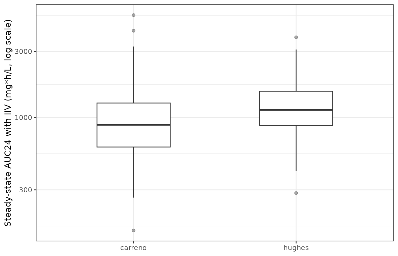
Between-subject spread of steady-state AUC24 in the BMI >= 40 cohort under the two models, with inter-individual variability switched on. The Carreno model’s much wider distribution is the flexibility Tong 2026 identifies as a source of unstable MAP estimates.
spread <- iiv |>
  dplyr::group_by(Model) |>
  dplyr::summarise(
    `median AUC24` = round(median(auc24), 1),
    `geometric CV %` = round(100 * sqrt(exp(var(log(auc24))) - 1), 1),
    `90% interval width / median` = round(
      diff(quantile(auc24, c(0.05, 0.95))) / median(auc24), 2),
    .groups = "drop"
  )
knitr::kable(spread, caption = paste(
  "Check 6. Between-subject dispersion of steady-state AUC24 under the two",
  "BMI >= 40 models. Reflects each model's published IIV structure:",
  "Carreno carries 55.6% CV on the renal clearance slope and 23.9% on the",
  "intercept; Hughes carries 21.8% CV on clearance."
))| Model | median AUC24 | geometric CV % | 90% interval width / median |
|---|---|---|---|
| carreno | 928.4 | 66.8 | 2.05 |
| hughes | 1140.0 | 46.6 | 1.63 |
# The Carreno model must be the more dispersed of the two -- that is the
# structural consequence of its variance terms, and the paper's argument.
carreno_cv <- spread$`geometric CV %`[spread$Model == "carreno"]
hughes_cv  <- spread$`geometric CV %`[spread$Model == "hughes"]
stopifnot(length(carreno_cv) == 1L, length(hughes_cv) == 1L,
          carreno_cv > hughes_cv)
Assumptions and deviations
Encoded as fixed priors throughout. Tong 2026
estimated no population parameters; the four models are priors for MAP
Bayesian estimation of individual parameters. Every ini()
entry is therefore wrapped in fixed(). This is directly
supported by the NONMEM FIX flags on the modified-Goti and
modified-Thomson streams. It is an inference, not a flag, for the other
two: the Carreno $OMEGA BLOCK(5) and all of the Hughes
$THETA and $OMEGA records except
THETA(7) carry no FIX flag in the supplement
listing, most likely because those records were pasted from the upstream
estimation control streams. Treating them as estimated would
misrepresent the study, in which they were held constant.
Variance convention is the control stream’s, not
log(CV^2 + 1). All four streams store omega values
that satisfy sqrt(omega^2) = %CV from Tables S1 and S2,
i.e. the omega^2 = CV^2 shorthand rather than the exact
log-normal omega^2 = log(CV^2 + 1). The control-stream
values are used verbatim, because they are the implemented model. This
is the main numerical difference from the sibling
Goti_2018_vancomycin extraction, which was made from the
Goti 2018 publication and applied the exact log-normal conversion
(0.14705 versus 0.1584 for clearance).
Differences from the existing
Goti_2018_vancomycin model file. The two are
deliberately not merged, because they are different models from
different sources. Beyond the variance convention above:
- Peripheral volume. The InsightRX stream sets
TVV2 = THETA(3)with no weight term, and Table S1 prints “V2 = 38.4”.Goti_2018_vancomycinscalesvpby(WT/70)on the strength of the Goti 2018 Methods statement that volume parameters were normalised to 70 kg. - Residual error. This implementation uses 1.42 mg/L additive and 19.7% proportional; Goti 2018 as published reports 3.4 mg/L and 22.7%.
- Creatinine clearance is computed inside the model here, and the elderly low-creatinine truncation described by Goti 2018 is absent – consistent with Tong 2021 (reference 19), which found that age-adjusting serum creatinine decreased predictive performance and was therefore not adopted.
Hughes proportional error: 0.1372 versus a tabulated
13.3%. The control stream gives $THETA(5) 0.1372
while Table S2 reports 13.3%. This is not a rounding difference. The
control-stream value is used as authoritative, on the grounds that it is
the machine-readable implemented model and is more precise; the
discrepancy is recorded here rather than silently reconciled. The
corresponding additive term, $THETA(6) 0.001 mg/L, is
effectively nil and is consistent with Table S2 printing “-” for that
row.
The Carreno peripheral transfer is routed through Q and
Vp. The Carreno $DES block drives the ODEs
directly from the micro-constants K12 and K21.
The model file keeps lk12 and lk21 as the
stored fixed effects, matching $THETA(3) and
$THETA(4), but computes q = k12 * vc and
vp = q / k21 and drives the ODEs from those. This is an
exact algebraic re-routing, not a change of model, and it is necessary:
written the literal way, rxSolve()’s
useLinCmt = TRUE rewrite drops peripheral1 and
silently solves a one-compartment model (terminal half-life 5.22 h
against a true 13.82 h, Cmax 52.8 against 27.1 mg/L). Because total AUC
is unaffected by that collapse, an exposure check would not reveal it,
so Check 1b asserts the half-life against the analytic beta root
instead.
The AUC accumulator compartment is omitted. Three of
the four streams declare a third state, DADT(3) = A(1)/V,
which integrates concentration to give AUC for MIPD reporting. It is a
quadrature accumulator, not a biological compartment: it has no analyte,
no specimen, and no influence on the PK. It is omitted from all four
model files, and AUC is obtained by NCA instead. Relatedly, the Hughes
stream uses the closed-form ADVAN3 TRANS4 and so has no
third state at all, yet its $ERROR block still assigns
AUC = A(3); that is a harmless leftover in the source
listing.
CL_HEMO is carried as
fixed(0). The modified-Goti and modified-Thomson
streams compute CLTOT = CL + CL_HEMO, where
CL_HEMO is a per-patient additive haemodialysis clearance
supplied by the MIPD software. Tong 2026 excluded haemodialysis patients
entirely, so it is identically zero throughout the study. Encoding it as
fixed(0) keeps the structural term visible and auditable
against the stream without inventing a covariate column for a quantity
the paper never varies.
Covariate polarity conversion. Both
internally-computing streams use SEX = 1 for male. The
canonical column is SEXF (1 = female), so
SEXF = 1 - SEX and the Cockcroft-Gault factor
0.85**(1-SEX) becomes 0.85^SEXF. The Hughes
stream’s IF(SEX.EQ.0) selection of the female Janmahasatian
coefficients independently confirms the polarity, so this is not an
assumption.
Creatinine clearance units. The InsightRX pipeline
supplies CRCL in L/h and both data-item streams convert to
mL/min inline (* 16.66667). These model files take
CRCL directly in mL/min, which is the scale on which the 66
mL/min centring value, the 150 mL/min cap and the 0.036 slope are all
expressed. CRCL here is raw Cockcroft-Gault creatinine
clearance and is not BSA-normalised, which the canonical
register permits with per-model documentation.
The virtual cohorts are marginal, not joint. Table 1 reports only a median and a min-max per covariate, so weight, age, sex and serum creatinine are simulated independently (log-normal for the positive continuous covariates, truncated to the published ranges) and height is fixed at the cohort median for the BMI < 40 arm, which does not use it. Real weight, age and creatinine are correlated, and the resulting creatinine-clearance distribution is therefore wider than the true one. Dosing is a flat 15 mg/kg q12h rounded to 250 mg, whereas the real cohort’s doses were individualised by MIPD. This is why Check 4 reproduces the direction and the asymmetry of the published a priori AUC disagreement but overstates its magnitude, and why that check bounds the mean difference loosely instead of asserting the published +17.5 mg*h/L. Checks 1, 2, 3 and 5 do not depend on the cohort construction: Checks 1 and 3 are deterministic algebra, and Checks 2 and 5 compare two quantities computed from the same drawn parameters, so their tolerances are tight by design.
Race and ethnicity are not reported in Tong 2026 for
either cohort and are absent from
population$race_ethnicity.
No published NCA table to compare against. Tong 2026
reports AUC target attainment and interrupted-time-series effect sizes,
not NCA summary statistics, so ncaComparisonTable() is not
used. Check 2 supplies the equivalent quantitative gate by comparing
PKNCA’s steady-state AUC against the exact Dose / CL identity for every
subject, and Check 1 pins every structural parameter against the printed
Table S1 / S2 equations.
Reference
Tong DMH, Brooks JT, Keizer RJ, Hughes JH. Vancomycin target attainment improved following population pharmacokinetic model switch: a large-scale quasi-experimental study of precision dosing. JAC Antimicrob Resist. 2026. doi:10.1093/jacamr/dlag016
Upstream model publications: Goti V et al. Ther Drug Monit 2018;40:212-221 (doi:10.1097/FTD.0000000000000490); Tong DMH et al. Ther Drug Monit 2021;43:139-140 (doi:10.1097/FTD.0000000000000819); Thomson AH et al. J Antimicrob Chemother 2009;63:1050-1057 (doi:10.1093/jac/dkp085); Carreno JJ et al. Antimicrob Agents Chemother 2017;61:e02478-16 (doi:10.1128/aac.02478-16); Hughes MSA et al. Ther Drug Monit 2024;46:575-583 (doi:10.1097/FTD.0000000000001214).