AZD7648 + olaparib xenograft PK-PD (DeJongh 2025)
Source:vignettes/articles/DeJongh_2025_azd7648_olaparib_xenograft.Rmd
DeJongh_2025_azd7648_olaparib_xenograft.RmdModels and source
This paper contributed three models, matching the three parameter tables and the three NONMEM control streams the authors published:
| Model | Source | What it is |
|---|---|---|
DeJongh_2025_azd7648_mouse |
Table 1 | AZD7648 population PK in mice |
DeJongh_2025_olaparib_mouse |
Table 2 | Olaparib population PK in mice |
DeJongh_2025_azd7648_olaparib_xenograft_mouse |
Tables 1-3 | The combined PK-PD tumour-growth-inhibition model |
- Article: https://doi.org/10.1007/s10928-025-09962-x
- Supplement (supplementary files 1-7, including the three NONMEM control streams, the tumour-static-equilibrium derivation and the PK-PD dataset): https://static-content.springer.com/esm/art%3A10.1007%2Fs10928-025-09962-x/MediaObjects/10928_2025_9962_MOESM4_ESM.txt
azd <- rxode2::rxode(readModelDb("DeJongh_2025_azd7648_mouse"))
#> ℹ parameter labels from comments will be replaced by 'label()'
ola <- rxode2::rxode(readModelDb("DeJongh_2025_olaparib_mouse"))
#> ℹ parameter labels from comments will be replaced by 'label()'
tgi <- rxode2::rxode(readModelDb("DeJongh_2025_azd7648_olaparib_xenograft_mouse"))
#> ℹ parameter labels from comments will be replaced by 'label()'- Citation: DeJongh J, Cadogan E, Davies M, Ramos-Montoya A, Smith A, van Steeg T, Richards R. (2025). Defining preclinical efficacy with the DNAPK inhibitor AZD7648 in combination with olaparib: a minimal systems pharmacokinetic-pharmacodynamic model. J Pharmacokinet Pharmacodyn 52:17. doi:10.1007/s10928-025-09962-x.
The authors fitted the two PK models on their own plasma datasets and
then carried only their fixed effects into the PK-PD
analysis, because most PK data came from satellite groups. The three
files reproduce that structure: the two PK models keep their
inter-individual variability and residual error, and the PK-PD model
wraps both PK models with every PK parameter fixed().
Population
str(tgi$population, max.level = 1)
#> List of 10
#>  $ species       : chr "mouse (female SCID C.B-17/IcrHan(R)Hsd-Prkdcscid bearing a subcutaneous FaDu ATM-knockout xenograft)"
#>  $ n_subjects    : int 120
#>  $ n_studies     : int 1
#>  $ age_range     : chr "at least 6 weeks of age at implantation"
#>  $ weight_range  : chr "(not reported in the source publication)"
#>  $ sex_female_pct: num 100
#>  $ disease_state : chr "subcutaneous FaDu ATM-knockout head-and-neck squamous-carcinoma xenograft in the dorsal left flank; randomised "| __truncated__
#>  $ dose_range    : chr "Study S1822 (model calibration): eight groups of 15 mice dosed orally once daily for 28 days with vehicle, AZD7"| __truncated__
#>  $ regions       : chr "preclinical (AstraZeneca, Cambridge UK; modelling by LAP&P Consultants, Leiden)"
#>  $ notes         : chr "Parameters in Table 3 were fitted simultaneously to all eight treatment groups of study S1822 (120 mice). Tumou"| __truncated__
AZD7648 and olaparib plasma PK were pooled from eight and six mouse studies respectively, in female SCID (C.B-17/IcrHan(R)Hsd-Prkdcscid) and female athymic nude (Hsd:Athymic Nude-Foxn1nu) mice at least six weeks old. Blood was drawn by tail-vein venipuncture (20 uL per sample, at most 100 uL over 24 h) and assayed by UPLC-MS/MS against an 11-point curve from 1 to 10,000 nM (LLOQ 0.009 nM).
The tumour PK-PD parameters (Table 3) were fitted simultaneously to all eight treatment groups of study S1822: 120 female SCID mice bearing a subcutaneous FaDu ATM-knockout xenograft, randomised at a mean tumour volume of about 0.2 cm3 and dosed orally once daily for 28 days with vehicle, AZD7648 monotherapy, olaparib monotherapy or one of five combinations, then followed through up to eight weeks of washout. Studies S1842 (six-week intermittent schedules) and S1826 were held out for a priori forecast evaluation and did not contribute to the estimates encoded here.
Amounts are molar. The supplied NONMEM dataset (supplementary file 7)
pairs each AMT in umol/kg with a DOSE in
mg/kg, which fixes the conversions used throughout this vignette:
UMOL_PER_MG_AZD <- 262.8812 / 100   # AZD7648: 100 mg/kg = 262.8812 umol/kg
UMOL_PER_MG_OLA <- 229.8428 / 100   # olaparib: 100 mg/kg = 229.8428 umol/kg
c(AZD7648 = 1000 / UMOL_PER_MG_AZD, olaparib = 1000 / UMOL_PER_MG_OLA)  # g/mol
#>  AZD7648 olaparib
#>   380.40   435.08
Source trace
Every ini() entry carries an in-file comment naming its
source location. The table below is the same trace in one place.
| Model | Quantity | Source |
|---|---|---|
| azd7648 | ka (SCID) 2.7726 1/h; ka (nude) 9.9 1/h | Table 1 |
| azd7648 | CL 0.251 L/kg/h; Vmax 4.27 umol/kg/h; Km 3.73 uM | Table 1 |
| azd7648 | Vc 3.45 L/kg (Vp = Vc); Q 0.932 L/kg/h | Table 1 |
| azd7648 | Nude relative F1 effect -0.520 | Table 1 |
| azd7648 | OMEGA block 0.0631 / -0.0291 / 0.193; prop. RE var 0.304 | Table 1 |
| azd7648 | Disposition equations | Equations 1-3 + supplementary file 5 $DES |
| olaparib | ka 10 1/h; CL 1.95 L/h; Vc 1.17 L/kg; Q 0.668 L/h; Vp 2.66 L/kg | Table 2 |
| olaparib | Per-study F1 0.425 / 0.174 / 0.489 / 0.598 / 0.238 / 1.48 / 4.18 | Table 2 + supplementary file 6 $THETA |
| olaparib | CmD50 82.5 mg/kg/day; OMEGA Vc 0.591; prop. RE var 0.399 | Table 2 |
| olaparib | Disposition + interaction equations | Equations 4-8 + supplementary file 6 $DES |
| xenograft | BL 0.115 cm3; GC 0.329 1/day; KC 2.25 cm3 | Table 3 |
| xenograft | AEC 1.93 mm3; G 0.637; Ktr 0.961 1/day | Table 3 |
| xenograft | EC50az 8.99 uM; EColap 0.0154 1/uM | Table 3 |
| xenograft | Kto = GC (not independently identifiable) | Table 3 footnote c |
| xenograft | OMEGA 0.0951 / 0.135 / 1.83 and 0.0362; prop. RE SD 0.243 | Table 3 |
| xenograft | Cell-state and biophase equations | Equations 9-18 + supplementary file 4 $DES |
| xenograft | Olaparib F1 = 4.1817 in the xenograft studies | supplementary file 4 (F11) |
| all | mg/kg to umol/kg conversions | supplementary file 7 (AMT vs DOSE columns) |
Part 1 - Pharmacokinetics
Replicating Figure 1
Figure 1 shows visual predictive checks after a single oral dose in SCID mice: 100 mg/kg AZD7648 alone (1a) and with 100 mg/kg olaparib (1b), and 100 mg/kg olaparib alone (1c) and with 100 mg/kg AZD7648 (1d). The single-dose SCID olaparib arms come from study S1734, so that study’s bioavailability factor applies.
N_PK <- 100L   # subjects per arm

# Both drugs absorb very fast (ka 2.8 and 10 1/h), so Tmax sits below an hour.
# The grid is deliberately dense over the first two hours: a coarser grid
# under-resolves the peak and the linear trapezoid then understates AUC by
# several percent, which would break the exact identity checked below.
PK_GRID <- c(seq(0, 2, by = 0.01), seq(2.1, 8, by = 0.1), seq(8.5, 72, by = 0.5))

pk_events <- function(n, dose_umol, cmt_dose, cmt_obs, covs) {
  doses <- tibble::tibble(id = seq_len(n), time = 0, amt = dose_umol,
                          evid = 1L, cmt = cmt_dose)
  obs <- tidyr::crossing(id = seq_len(n), time = PK_GRID) |>
    mutate(amt = NA_real_, evid = 0L, cmt = cmt_obs)
  ev <- bind_rows(doses, obs) |> arrange(id, time, desc(evid))
  for (nm in names(covs)) ev[[nm]] <- covs[[nm]]
  ev
}

# --- AZD7648: identical with and without olaparib (no reverse interaction) ---
ev_azd <- pk_events(N_PK, 100 * UMOL_PER_MG_AZD, "depot", "central",
                    list(STRAIN_NUDE = 0))
sim_azd <- rxode2::rxSolve(azd, ev_azd, useLinCmt = FALSE,
                           returnType = "data.frame")
stopifnot(dplyr::n_distinct(sim_azd$id) == N_PK)

# --- Olaparib: monotherapy vs 100 mg/kg/day AZD7648 co-treatment ---
ola_covs <- function(dazd) {
  list(STRAIN_NUDE = 0, STUDY_S1143 = 0, STUDY_S1721 = 0, STUDY_S1734 = 1,
       STUDY_S1770 = 0, STUDY_S1816 = 0, DOSE_AZD7648_MGKGD = dazd)
}
sim_ola <- bind_rows(lapply(c(0, 100), function(dz) {
  ev <- pk_events(N_PK, 100 * UMOL_PER_MG_OLA, "depot", "central", ola_covs(dz))
  rxode2::rxSolve(ola, ev, useLinCmt = FALSE, returnType = "data.frame") |>
    mutate(arm = if (dz == 0) "olaparib alone" else "olaparib + AZD7648")
}))
stopifnot(dplyr::n_distinct(sim_ola$id) == N_PK)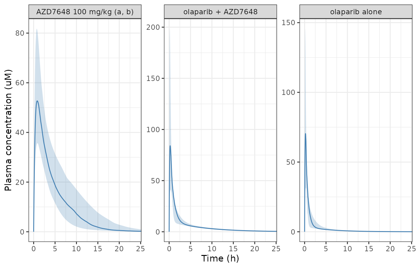
Replicates Figure 1 of DeJongh 2025: single-dose plasma profiles in SCID mice. Ribbons are the 10-90% prediction interval, lines the median.
Co-treatment raises olaparib exposure, which is the PK half of the paper’s explanation for the combination’s efficacy. AZD7648 is unchanged by olaparib: the interaction in this model runs in one direction only.
PKNCA
nca_one <- function(sim, dose_umol, label) {
  conc <- sim |> filter(!is.na(Cc)) |> transmute(id, time, Cc, arm = label)
  dose <- conc |> distinct(id, arm) |> mutate(time = 0, amt = dose_umol)
  o <- PKNCA::pk.nca(PKNCA::PKNCAdata(
    PKNCA::PKNCAconc(conc, Cc ~ time | arm + id, concu = "uM", timeu = "h"),
    PKNCA::PKNCAdose(dose, amt ~ time | arm + id, doseu = "umol/kg"),
    intervals = data.frame(start = 0, end = Inf, cmax = TRUE, tmax = TRUE,
                           aucinf.obs = TRUE, half.life = TRUE)))
  as.data.frame(o$result)
}
nca <- bind_rows(
  nca_one(sim_azd, 100 * UMOL_PER_MG_AZD, "AZD7648 100 mg/kg"),
  nca_one(filter(sim_ola, arm == "olaparib alone"), 100 * UMOL_PER_MG_OLA,
          "olaparib 100 mg/kg"),
  nca_one(filter(sim_ola, arm == "olaparib + AZD7648"), 100 * UMOL_PER_MG_OLA,
          "olaparib 100 mg/kg + AZD7648")
)| Arm | adj.r.squared | AUC0-inf (uM*h) | clast.obs | clast.pred | Cmax (uM) | t1/2 (h) | lambda.z | lambda.z.n.points | lambda.z.time.first | lambda.z.time.last | r.squared | span.ratio | tlast | Tmax (h) |
|---|---|---|---|---|---|---|---|---|---|---|---|---|---|---|
| AZD7648 100 mg/kg | 1 | 261.234 | 0.000 | 0.000 | 52.706 | 3.260 | 0.213 | 112.0 | 16.50 | 72 | 1 | 16.726 | 72 | 0.84 |
| olaparib 100 mg/kg | 1 | 70.568 | 0.000 | 0.000 | 70.413 | 3.830 | 0.181 | 185.0 | 2.40 | 72 | 1 | 18.173 | 72 | 0.20 |
| olaparib 100 mg/kg + AZD7648 | 1 | 156.077 | 0.001 | 0.001 | 84.059 | 5.297 | 0.131 | 177.5 | 3.15 | 72 | 1 | 12.998 | 72 | 0.24 |
DeJongh 2025 reports no NCA table, so there is nothing to compare these against directly. Instead the model is checked against three identities that follow exactly from the published parameters.
Check 1 - olaparib AUC equals F x Dose / CL
Olaparib elimination is linear, so AUC(0-inf) must equal
F * Dose / CL exactly, per subject. The one random effect
is on Vc, which does not enter that identity, so every subject must
agree to solver tolerance.
F_S1734_SCID <- 0.59754; CL_OLA <- 1.9460
expected <- F_S1734_SCID * 100 * UMOL_PER_MG_OLA / CL_OLA
observed <- nca |> filter(arm == "olaparib 100 mg/kg", PPTESTCD == "aucinf.obs")
stopifnot(nrow(observed) == N_PK)
rel_err <- abs(observed$PPORRES - expected) / expected
c(expected = expected, max_rel_error = max(rel_err))
#>      expected max_rel_error
#>  7.057568e+01  8.921745e-04
stopifnot(max(rel_err) < 0.002)
Check 2 - the interaction halves clearance at CmD50
CmD50 = 82.5 mg/kg/day is defined as the AZD7648 daily
dose that reduces olaparib clearance by 50%. At that dose olaparib AUC
must therefore be exactly doubled.
auc_at <- function(dazd) {
  ev <- pk_events(50L, 100 * UMOL_PER_MG_OLA, "depot", "central", ola_covs(dazd))
  s <- rxode2::rxSolve(rxode2::zeroRe(ola), ev, omega = NA, useLinCmt = FALSE,
                       returnType = "data.frame")
  n <- nca_one(s, 100 * UMOL_PER_MG_OLA, "x")
  median(n$PPORRES[n$PPTESTCD == "aucinf.obs"])
}
ratio <- auc_at(82.538) / auc_at(0)
#> Warning: multi-subject simulation without without 'omega'
#> Warning: multi-subject simulation without without 'omega'
c(auc_ratio = ratio, expected = 2)
#> auc_ratio  expected
#>  2.000171  2.000000
stopifnot(abs(ratio - 2) < 0.01)
Check 3 - AZD7648 elimination is saturable
With a Michaelis-Menten term alongside linear clearance, dose-normalised exposure must rise with dose.
dnauc <- vapply(c(25, 50, 100, 150), function(d) {
  ev <- pk_events(1L, d * UMOL_PER_MG_AZD, "depot", "central",
                  list(STRAIN_NUDE = 0))
  s <- rxode2::rxSolve(rxode2::zeroRe(azd), ev, omega = NA, useLinCmt = FALSE,
                       returnType = "data.frame")
  if (is.null(s$id)) s$id <- 1L
  n <- nca_one(s, d * UMOL_PER_MG_AZD, "x")
  n$PPORRES[n$PPTESTCD == "aucinf.obs"] / (d * UMOL_PER_MG_AZD)
}, numeric(1))
names(dnauc) <- paste0(c(25, 50, 100, 150), " mg/kg")
round(dnauc, 4)
#>  25 mg/kg  50 mg/kg 100 mg/kg 150 mg/kg
#>    0.5284    0.7389    1.0576    1.3046
stopifnot(all(diff(dnauc) > 0))
Part 2 - The tumour PK-PD model
Check 4 - the untreated steady state
Supplementary file 2 derives the untreated steady state analytically.
With Kto = GC and the Allee factor at its high-mass limit
of 1, total tumour volume settles at exactly the carrying capacity
KC, and the four cell states hold 40% / 20% / 20% / 20% of
it.
ev_ss <- tibble::tibble(id = 1L, time = seq(0, 365 * 24, by = 24),
                        amt = NA_real_, evid = 0L, cmt = "cycling_cells",
                        DOSE_AZD7648_MGKGD = 0)
ss <- rxode2::rxSolve(rxode2::zeroRe(tgi), ev_ss, omega = NA,
                      useLinCmt = FALSE, returnType = "data.frame") |> tail(1)
fractions <- with(ss, c(proliferating = cycling_cells, quiescent = damaged_cells1,
                        dying1 = damaged_cells2, dying2 = damaged_cells3) /
                    tumor_size)
round(fractions, 4)
#> proliferating     quiescent        dying1        dying2
#>           0.4           0.2           0.2           0.2
stopifnot(max(abs(fractions - c(0.4, 0.2, 0.2, 0.2))) < 0.002)
The realised steady state sits just below KC because the
Allee factor is 0.98, not 1, at that tumour size. Retaining it gives the
exact balance condition
(1 - Atot / (2 KC)) * AlleeEff = 1/2:
AEC_CM3 <- 1.93 / 1000; G_HILL <- 0.637; KC <- 2.25
allee <- with(ss, cycling_cells^G_HILL / (cycling_cells^G_HILL + AEC_CM3^G_HILL))
balance <- (1 - ss$tumor_size / (2 * KC)) * allee
c(tumor_size = ss$tumor_size, KC_limit = KC, allee_factor = allee,
  balance = balance, expected = 0.5)
#>   tumor_size     KC_limit allee_factor      balance     expected
#>    2.2045138    2.2500000    0.9801845    0.5000000    0.5000000
stopifnot(abs(balance - 0.5) < 1e-3)
Replicating Figures 2 and 3 - study S1822
The eight treatment groups of study S1822, all dosed once daily for 28 days (olaparib one hour after the morning AZD7648 dose). Observed medians are read from the supplied PK-PD dataset (supplementary file 7).
groups <- tibble::tribble(
  ~grp, ~azd, ~ola, ~label,
  1L,   0,    0,    "1: vehicle",
  2L, 100,    0,    "2: AZD 100",
  3L, 100,  100,    "3: AZD 100 + Ola 100",
  4L, 100,   50,    "4: AZD 100 + Ola 50",
  5L,  50,   50,    "5: AZD 50 + Ola 50",
  6L,  50,  100,    "6: AZD 50 + Ola 100",
  7L,   0,  100,    "7: Ola 100",
  8L,  75,   75,    "8: AZD 75 + Ola 75")

tgi_events <- function(id, azd, ola, days = 77, by = 12) {
  obs <- tibble::tibble(time = seq(0, days * 24, by = by), amt = NA_real_,
                        evid = 0L, cmt = "cycling_cells", ii = 0, addl = 0)
  d <- NULL
  if (azd > 0) d <- bind_rows(d, tibble::tibble(time = 0, amt = azd * UMOL_PER_MG_AZD,
                    evid = 1L, cmt = "depot", ii = 24, addl = 27))
  if (ola > 0) d <- bind_rows(d, tibble::tibble(time = 1, amt = ola * UMOL_PER_MG_OLA,
                    evid = 1L, cmt = "depot_olaparib", ii = 24, addl = 27))
  bind_rows(d, obs) |> arrange(time, desc(evid)) |>
    mutate(id = id, DOSE_AZD7648_MGKGD = azd)
}

ev_typ <- purrr::map_dfr(seq_len(nrow(groups)),
                         \(i) tgi_events(groups$grp[i], groups$azd[i], groups$ola[i]))
sim_typ <- rxode2::rxSolve(rxode2::zeroRe(tgi), ev_typ, omega = NA,
                           useLinCmt = FALSE, returnType = "data.frame") |>
  left_join(groups, by = c("id" = "grp"))
#> Warning: multi-subject simulation without without 'omega'
stopifnot(dplyr::n_distinct(sim_typ$id) == 8L)
observed <- tibble::tribble(
  ~grp, ~day, ~tv,
  1L,0,0.1196, 1L,7,0.4843, 1L,9,0.5682, 1L,14,0.6735, 1L,18,0.7746, 1L,21,1.5365,
  2L,0,0.1263, 2L,7,0.3608, 2L,9,0.3960, 2L,14,0.5236, 2L,18,0.7342, 2L,21,0.9571,
  3L,0,0.1263, 3L,7,0.2989, 3L,9,0.2917, 3L,14,0.2038, 3L,18,0.1781, 3L,21,0.0908,
  3L,28,0.0965, 3L,35,0.0397, 3L,42,0.0494, 3L,49,0.0486, 3L,56,0.0702, 3L,63,0.0985,
  3L,70,0.1692, 3L,77,0.3459,
  4L,0,0.1263, 4L,7,0.2833, 4L,9,0.3274, 4L,14,0.2665, 4L,18,0.2285, 4L,21,0.1716,
  4L,28,0.2333, 4L,35,0.1498, 4L,42,0.2729, 4L,49,0.6485, 4L,56,0.6459, 4L,63,0.9852,
  5L,0,0.1251, 5L,7,0.4024, 5L,9,0.4259, 5L,14,0.4416, 5L,18,0.4952, 5L,21,0.4798,
  5L,28,0.7619,
  6L,0,0.1259, 6L,7,0.2575, 6L,9,0.2652, 6L,14,0.2514, 6L,18,0.2285, 6L,21,0.2238,
  6L,28,0.3862, 6L,35,0.3138, 6L,42,0.6544, 6L,49,0.8796, 6L,56,1.0379,
  7L,0,0.1250, 7L,7,0.3742, 7L,9,0.4203, 7L,14,0.4915, 7L,18,0.5179, 7L,21,0.6579,
  7L,28,1.2893,
  8L,0,0.1254, 8L,7,0.3289, 8L,9,0.3124, 8L,14,0.2678, 8L,18,0.2227, 8L,21,0.1511,
  8L,28,0.2070, 8L,35,0.2269, 8L,42,0.4955, 8L,49,0.7412, 8L,56,1.2251, 8L,63,0.6633,
  8L,70,1.5712) |>
  left_join(groups, by = "grp")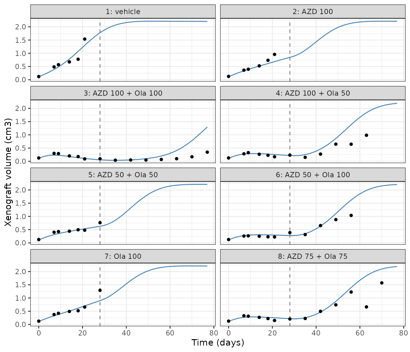
Replicates Figures 2a and 3b of DeJongh 2025: observed median xenograft volume (points, supplementary file 7) against the typical-value prediction of the packaged model (lines). The vertical line marks the end of the 28-day treatment period.
The model reproduces the qualitative pattern the paper describes: monotherapy with either agent slows growth but never drives the tumour below baseline, whereas every combination arm regresses below the pre-treatment volume, with delayed re-growth after treatment stops. Agreement is closest during the 28-day treatment period. Median observed volumes in the washout phase rest on progressively fewer animals (as few as one or two by day 63-70) because of the non-random dropout the paper discusses in its Discussion, so the late points should not be read as a like-for-like comparison.
| Group | Day | Observed median (cm3) | Model typical value (cm3) | Ratio |
|---|---|---|---|---|
| 1: vehicle | 21 | 1.536 | 1.300 | 0.85 |
| 2: AZD 100 | 21 | 0.957 | 0.683 | 0.71 |
| 3: AZD 100 + Ola 100 | 21 | 0.091 | 0.108 | 1.19 |
| 3: AZD 100 + Ola 100 | 28 | 0.096 | 0.057 | 0.59 |
| 4: AZD 100 + Ola 50 | 21 | 0.172 | 0.257 | 1.50 |
| 4: AZD 100 + Ola 50 | 28 | 0.233 | 0.220 | 0.94 |
| 5: AZD 50 + Ola 50 | 21 | 0.480 | 0.534 | 1.11 |
| 5: AZD 50 + Ola 50 | 28 | 0.762 | 0.628 | 0.82 |
| 6: AZD 50 + Ola 100 | 21 | 0.224 | 0.295 | 1.32 |
| 6: AZD 50 + Ola 100 | 28 | 0.386 | 0.278 | 0.72 |
| 7: Ola 100 | 21 | 0.658 | 0.700 | 1.06 |
| 7: Ola 100 | 28 | 1.289 | 0.901 | 0.70 |
| 8: AZD 75 + Ola 75 | 21 | 0.151 | 0.253 | 1.67 |
| 8: AZD 75 + Ola 75 | 28 | 0.207 | 0.218 | 1.05 |
The Allee effect and sustained regression
The paper’s central structural claim is that an Allee term is needed to explain why a minority of mice regress permanently while most re-grow. With inter-individual variability switched on, the packaged model reproduces that split in the highest-dose combination group.
N_TGI <- 100L
ev_pop <- purrr::map_dfr(seq_len(N_TGI), \(i) tgi_events(i, 100, 100))
sim_pop <- rxode2::rxSolve(tgi, ev_pop, useLinCmt = FALSE,
                           returnType = "data.frame")
stopifnot(dplyr::n_distinct(sim_pop$id) == N_TGI)

# The typical-value chunks above pass zeroRe(tgi) into rxSolve(). That call
# mutates state shared with the model object, and a silent strip would collapse
# this cohort to 100 identical animals without raising an error. Recover the
# two random effects from the returned per-subject parameters and check them
# against the Table 3 omegas, so the failure cannot pass unnoticed.
etas <- distinct(sim_pop, id, rbase, kge)
stopifnot(
  nrow(etas) == N_TGI,
  abs(sd(log(etas$rbase)) - sqrt(0.0951)) < 0.10,   # Om_1 (BL)
  abs(sd(log(etas$kge))   - sqrt(0.0362)) < 0.10    # Om_3 (GC)
)

final <- sim_pop |> filter(time == max(time)) |>
  transmute(id, tumor_size, regressed = tumor_size < 0.05)
mean(final$regressed)
#> [1] 0.35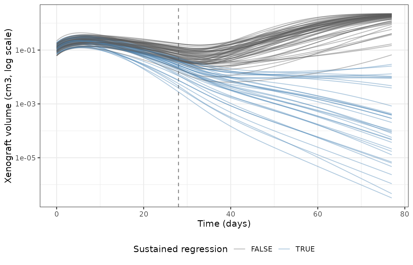
Replicates Figure 3b of DeJongh 2025: individual profiles in the 100 mg/kg AZD7648 + 100 mg/kg olaparib group. Blue traces are animals in sustained regression at the end of follow-up; the Allee term is what allows the two outcomes to coexist under identical dosing.
Replicating Figures 4 and 5 - the a priori forecast for study S1842
Study S1842 was held out of the fit: the model was calibrated on 28 days of continuous dosing in S1822 and then used to forecast six weeks of intermittent schedules. All seven treated groups received 100 mg/kg olaparib once daily throughout; AZD7648 was given twice daily at 75 or 37.5 mg/kg under a continuous or an on/off schedule (Table S1). Figures 4 and 5 of the paper are built from these groups, so they are reproduced here rather than from S1822.
on_days <- function(sched) {
  d <- 0:41
  switch(sched,
    continuous = d,
    `14/14/14` = d[(d < 14) | (d >= 28)],
    `7/7`      = d[(d %% 14) < 7],
    `5/2`      = d[(d %%  7) < 5],
    `3/4`      = d[(d %%  7) < 3])
}
s1842 <- tibble::tribble(
  ~grp, ~azd_bid, ~sched,       ~label,
  2L,   75,       "continuous", "AZD 75 continuous",
  3L,   75,       "14/14/14",   "AZD 75 14/14/14",
  4L,   75,       "7/7",        "AZD 75 7/7",
  5L,   75,       "5/2",        "AZD 75 5/2",
  6L,   75,       "3/4",        "AZD 75 3/4",
  7L,   37.5,     "continuous", "AZD 37.5 continuous",
  8L,   37.5,     "5/2",        "AZD 37.5 5/2")

s1842_events <- function(id, azd_bid, sched) {
  onl <- on_days(sched)
  # AZD7648 twice daily (0 and 12 h) on treatment days only
  azd_d <- tidyr::crossing(day = onl, h = c(0, 12)) |>
    transmute(time = day * 24 + h, amt = azd_bid * UMOL_PER_MG_AZD,
              evid = 1L, cmt = "depot")
  # olaparib once daily throughout, 1 h after the morning AZD7648 dose
  ola_d <- tibble::tibble(time = (0:41) * 24 + 1, amt = 100 * UMOL_PER_MG_OLA,
                          evid = 1L, cmt = "depot_olaparib")
  obs <- tibble::tibble(time = seq(0, 42 * 24, by = 6), amt = NA_real_,
                        evid = 0L, cmt = "cycling_cells")
  bind_rows(azd_d, ola_d, obs) |> arrange(time, desc(evid)) |>
    mutate(id = id, .day = floor(time / 24),
           # the interaction is driven by the AZD7648 dose actually given that
           # day, so the covariate drops to 0 during an off-period
           DOSE_AZD7648_MGKGD = ifelse(.day %in% onl, 2 * azd_bid, 0)) |>
    select(-.day)
}
ev_1842 <- purrr::map_dfr(seq_len(nrow(s1842)),
                          \(i) s1842_events(s1842$grp[i], s1842$azd_bid[i], s1842$sched[i]))
sim_1842 <- rxode2::rxSolve(rxode2::zeroRe(tgi), ev_1842, omega = NA,
                            useLinCmt = FALSE, returnType = "data.frame") |>
  left_join(s1842, by = c("id" = "grp"))
#> Warning: multi-subject simulation without without 'omega'
stopifnot(dplyr::n_distinct(sim_1842$id) == 7L)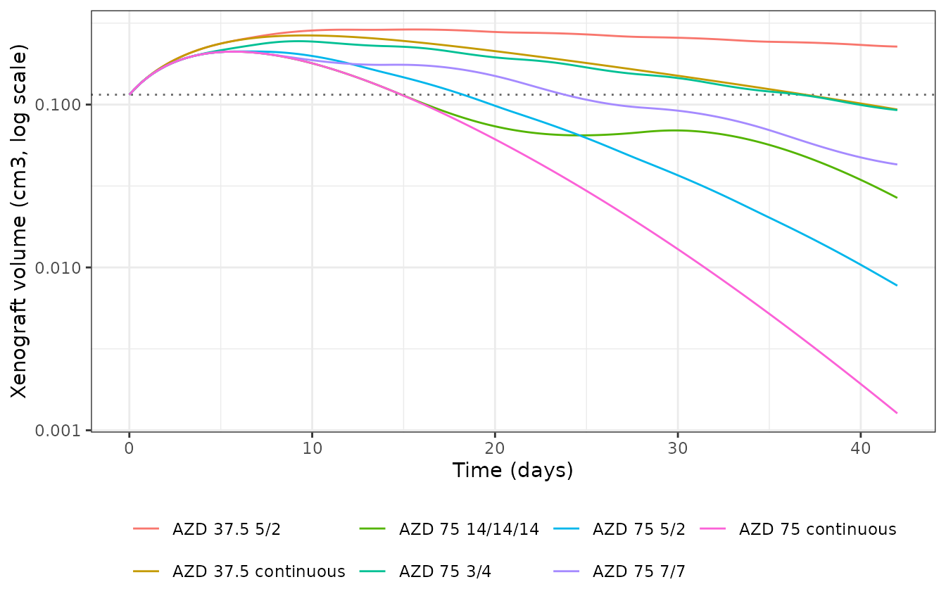
Replicates Figure 4 of DeJongh 2025: a priori forecasts of xenograft volume for the six-week intermittent schedules of study S1842, a dataset held out of the model fit.
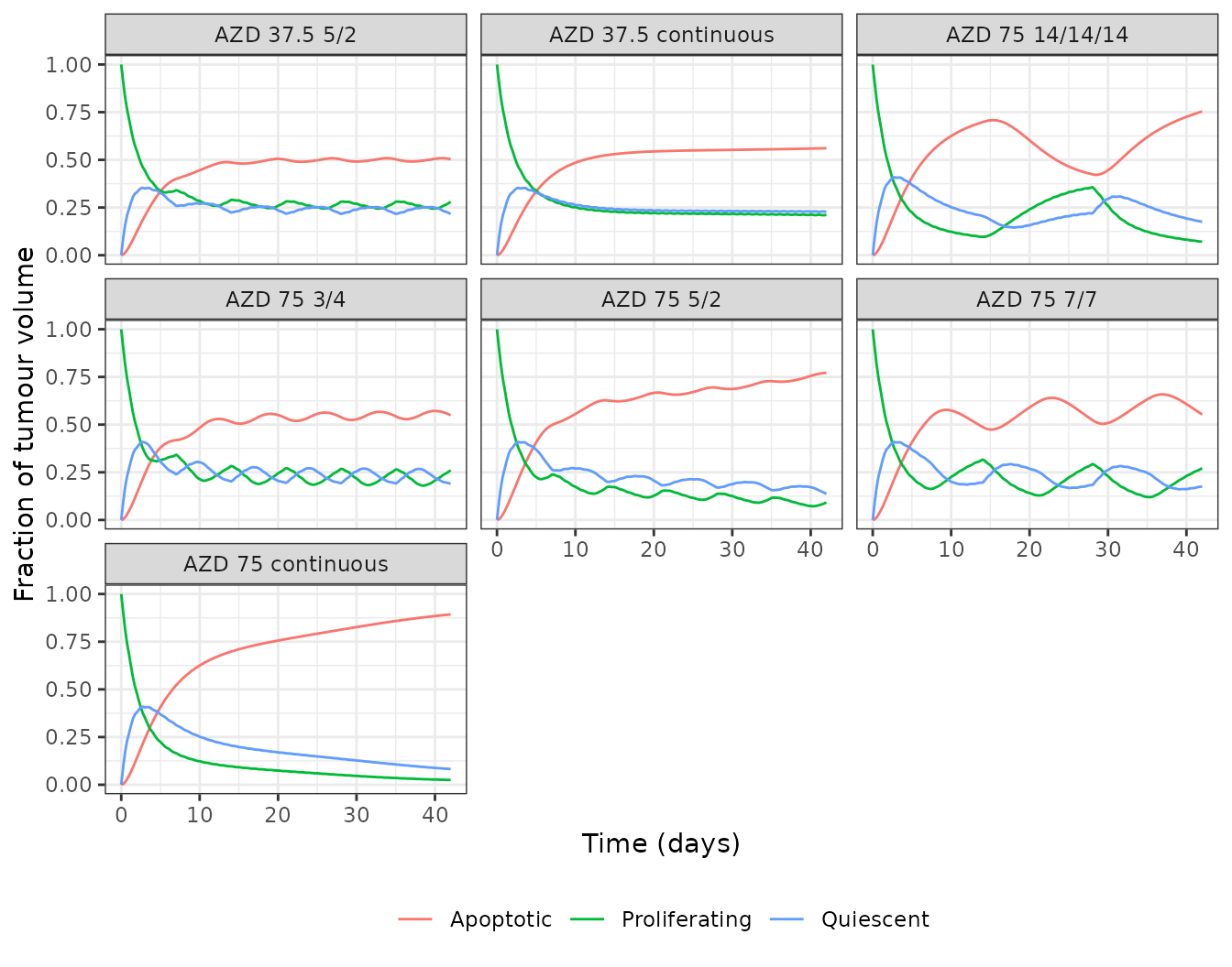
Replicates Figure 5a of DeJongh 2025: fractional occupancy of each cell state over the six-week treatment period.
trapz <- function(t, y) sum(diff(t) * (head(y, -1) + tail(y, -1)) / 2)

occupancy <- sim_1842 |>
  group_by(grp = id, label) |>
  summarise(
    prol      = trapz(time, cycling_cells / tumor_size),
    quiesc    = trapz(time, damaged_cells1 / tumor_size),
    apop      = trapz(time, (damaged_cells2 + damaged_cells3) / tumor_size),
    max_apop  = max((damaged_cells2 + damaged_cells3) / tumor_size),
    prol_depl = 1 - min(cycling_cells / tumor_size),
    # Figure 5b efficacy: fold change 24 h after the last dose vs baseline
    fold      = tumor_size[which.max(time)] / first(tumor_size),
    .groups   = "drop") |>
mutate(ratio = apop / prol)| Schedule | Max apoptotic fraction | Proliferating depletion | Apoptotic:proliferating AUC ratio | Fold change vs baseline |
|---|---|---|---|---|
| AZD 75 continuous | 0.893 | 0.975 | 5.67 | 0.011 |
| AZD 75 5/2 | 0.771 | 0.928 | 3.41 | 0.067 |
| AZD 75 14/14/14 | 0.754 | 0.928 | 2.47 | 0.232 |
| AZD 75 7/7 | 0.658 | 0.880 | 2.20 | 0.373 |
| AZD 75 3/4 | 0.572 | 0.820 | 1.83 | 0.804 |
| AZD 37.5 continuous | 0.561 | 0.790 | 1.82 | 0.811 |
| AZD 37.5 5/2 | 0.509 | 0.756 | 1.46 | 1.975 |
The paper makes four quantitative statements about these panels; each is checked below.
# "All groups achieved apoptotic fractions > 50% during the treatment period"
stopifnot(nrow(occupancy) == 7L, all(occupancy$max_apop > 0.50))

# "Both 37.5 mg/kg groups (continuous, 5/2) sustained an apoptotic fraction < 60%"
low_dose <- occupancy$max_apop[occupancy$grp %in% c(7L, 8L)]
stopifnot(length(low_dose) == 2L, all(low_dose < 0.60))

# "Sustained regression occurred in individual mice under most intermittent
#  75 mg/kg regimens, but not at a 3 day on/4 day off schedule or at the
#  37.5 mg/kg dose level" -- exactly the > 2:1 apoptotic:proliferating split.
sustained <- occupancy$ratio[occupancy$grp %in% c(2L, 3L, 4L, 5L)]
not_sustained <- occupancy$ratio[occupancy$grp %in% c(6L, 7L, 8L)]
stopifnot(length(sustained) == 4L, length(not_sustained) == 3L)
stopifnot(min(sustained) > 2, max(not_sustained) < 2)

# "Linear relationships were observed between efficacy [...] and fractional
#  populations in proliferative (R2 = 0.97) and apoptotic (R2 = 0.93)
#  fractions, but not for the quiescent population (R2 = 0.42)"
r2 <- c(proliferating = cor(occupancy$prol,   occupancy$fold)^2,
        apoptotic     = cor(occupancy$apop,   occupancy$fold)^2,
        quiescent     = cor(occupancy$quiesc, occupancy$fold)^2)
round(r2, 3)
#> proliferating     apoptotic     quiescent
#>         0.706         0.631         0.403
stopifnot(r2[["quiescent"]] < r2[["apoptotic"]],
          r2[["quiescent"]] < r2[["proliferating"]],
          abs(r2[["quiescent"]] - 0.42) < 0.10)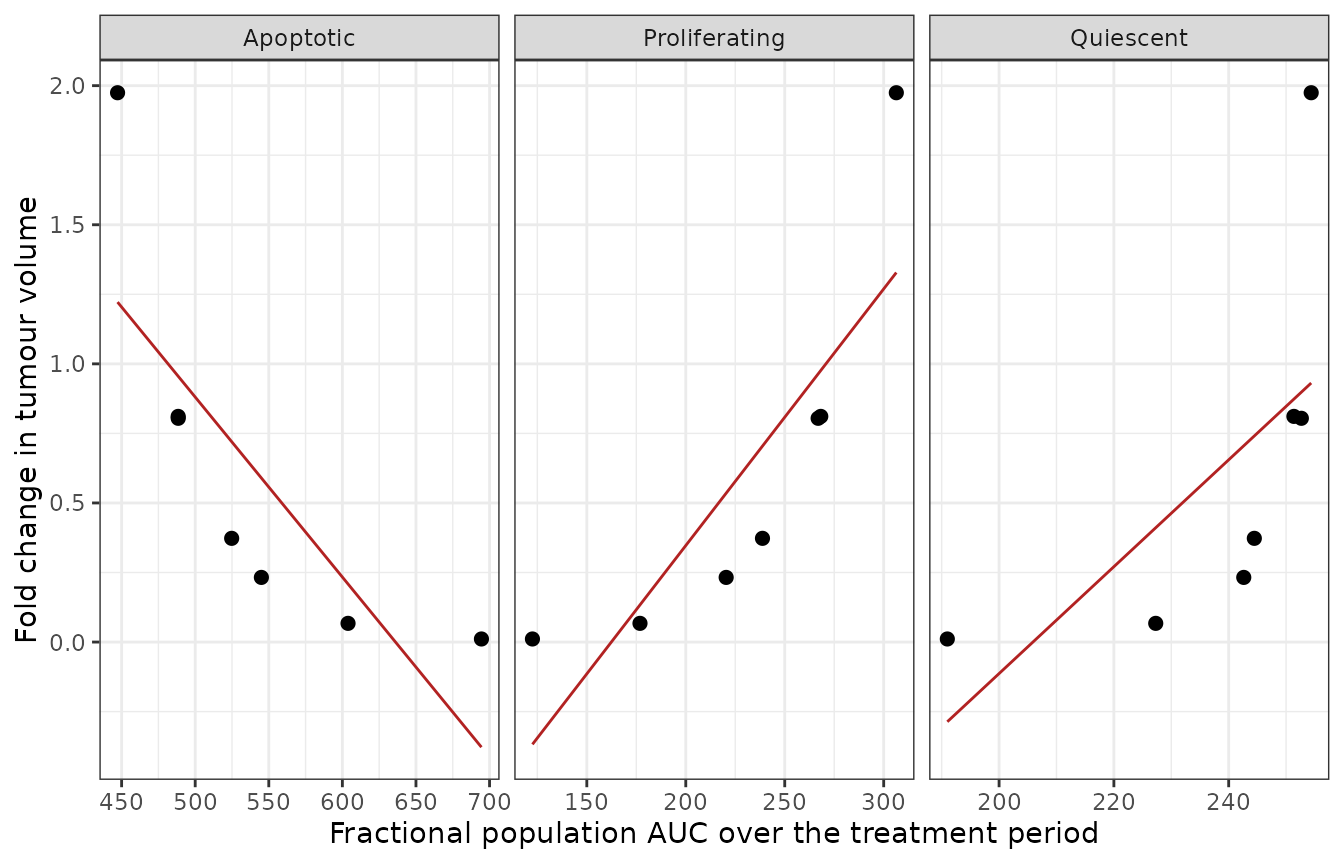
Replicates Figure 5b of DeJongh 2025: efficacy (fold change from baseline 24 h after the last dose) against the fractional-population AUC of each cell state.
The ordering the paper reports is recovered: proliferating and apoptotic fractions both track efficacy closely, the quiescent fraction much less so, and the model’s quiescent R2 lands within 0.03 of the published 0.42. The apoptotic:proliferating ratio separates the four schedules the paper reports as achieving sustained regression from the three it reports as failing, at exactly the published 2:1 threshold.
Check 5 - the tumour static equilibrium (Figure S10)
The supplementary derivation gives the tumour-static-equilibrium
condition in closed form. Writing the two drug effects as
w = 1 + EColap * C_olap and
a = 1 - C_az / (C_az + EC50az), stasis at negligible
baseline volume requires w = 1 + a, i.e.
EColap * C_olap = 1 - C_az / (C_az + EC50az).
ECOLAP <- 0.0154; EC50AZ <- 8.99
tse_olaparib <- function(c_az) (1 - c_az / (c_az + EC50AZ)) / ECOLAP
published <- tibble::tribble(
  ~Claim,                                        ~Published, ~Model,
  "Olaparib alone, TSE concentration (uM)",           64.9,  tse_olaparib(0),
  "Olaparib TSE at 20.2 uM AZD7648 (uM)",             19.9,  tse_olaparib(20.2)
)
stopifnot(with(published, max(abs(Model - Published) / Published)) < 0.01)| Quantity | DeJongh 2025 | Packaged model | Difference (%) |
|---|---|---|---|
| Olaparib alone, TSE concentration (uM) | 64.9 | 64.94 | 0.1 |
| Olaparib TSE at 20.2 uM AZD7648 (uM) | 19.9 | 20.00 | 0.5 |
AZD7648 monotherapy can never reach the equilibrium: with
C_olap = 0 the left-hand side is 0 while the right-hand
side is strictly positive for any finite AZD7648 concentration. That
reproduces the paper’s statement that “AZD7648 is unable to achieve TSE
as a monotherapy”.
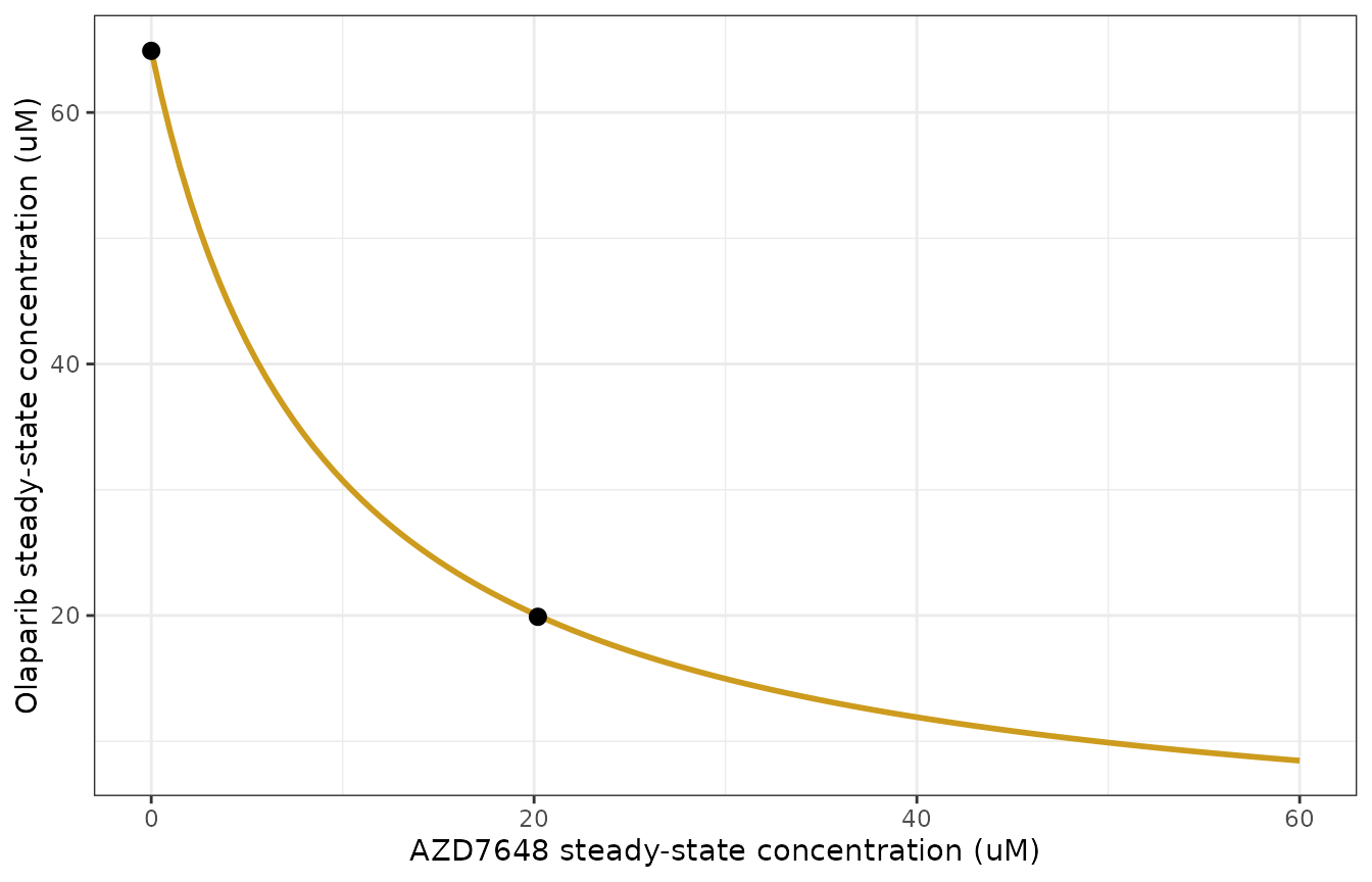
Replicates Figure S10 of DeJongh 2025: the tumour static equilibrium nomogram. Concentration pairs above the curve drive regression; pairs below it are insufficient for stasis.
Assumptions and deviations
Errata against the published equations. Three printed equations disagree with the NONMEM control streams the authors supplied. In each case the control stream is authoritative and is what the packaged models implement, because the control streams are what produced the published parameter estimates and figures.
Equation 1, Michaelis-Menten elimination. As printed, the saturable term is
Vmax / (A1/Vc + Km), which has units of a clearance rather than a rate and would not balance the equation. Both AZD7648 control streams (supplementary files 4 and 5) codeVmax*A(2)/(A(2)/Vc + Km). The amount in the numerator was dropped in typesetting.Equation 16, the olaparib effect. As printed,
OlEff = Ce,Olap * EColap. The control stream codesOLEFF = 1 + ECol*COL. The leading 1 is the untreated baseline flux between the proliferating and quiescent states; without it vehicle animals would have no cell cycling at all, the untreated steady state derived in supplementary file 2 would not exist, and the 40/20/20/20 split reproduced in Check 4 above would be unreachable.Equation 10, the logistic limitation term. The printed form reads as
1 - (1 - Kto/2) * TXeno/KC. The control stream codes1 - Atot/(2*KC), which is also the form used in the supplementary steady-state derivation.
Residual numerical differences. Two Figure 5a numbers do not match exactly. The paper reports a maximum apoptotic fraction “> 70%” for the 75 mg/kg 7 on / 7 off schedule and 67% for the 3 on / 4 off schedule; the packaged model gives 66% and 57%. Every other statement about that panel reproduces (all groups above 50%, both 37.5 mg/kg groups below 60%, proliferating depletion above 90% for the continuous / 14-14-14 / 5-2 schedules). The 3 on / 4 off group is also the one the paper singles out as its poorest forecast, so some of the gap is likely the same phenomenon. No parameter was adjusted to close it.
Table labelling. Table 2’s “Absolute bio-avail F1 =
0.598” row is the study S1734 SCID factor (control stream
THETA(10)); the value anchored on the intravenous arm is
the 0.425 entry labelled “F1 11,448 (Nude)” (THETA(7),
commented “abs F1, based on 11448”). Table 3’s Kto row
carries the abbreviation and units but no value, with 0.243 printed on
the following “Proportional residual error” line; footnote c supplies
Kto = GC.
Residual-error scale. Tables 1 and 2 label the
proportional residual error as a variance and the control streams
confirm it (W = IPRED*SQRT(THETA)), so those models use
sqrt(0.304) and sqrt(0.399). Table 3 gives no
such label, and its control stream uses W = IPRED*THETA(9)
with $SIGMA 1 FIX, so 0.243 is a standard deviation and is
used unchanged. Getting this wrong in either direction would misstate
the residual magnitude by roughly a factor of two.
Unit conventions carried as published. Olaparib
clearance and intercompartmental clearance are reported in L/h while its
volumes are in L/kg. The rate constants the model actually integrates
are unaffected, and the scale mismatch is absorbed into the per-study
bioavailability factors - which is why some exceed 1 (S1770 = 1.48,
S1816 = 4.18). These are descriptive inter-study scaling factors, not
physiological bioavailabilities. Similarly, the AZD7648
Vmax of 4.27 umol/kg/h enters the saturable term multiplied
by the central amount rather than the concentration, so it is not a
maximum elimination rate in the usual dimensional sense; it is
transcribed exactly as coded.
Assumptions the source made explicit.
Vp = Vc for AZD7648 (Table 1); ka = 9.9 1/h
for AZD7648 in nude mice and ka = 10 1/h for olaparib, both
fixed for want of absorption-phase data; Kto = GC (Table 3
footnote c); and all tumour cells proliferating at study start, which
the control stream notes has “very limited sensitivity on GoF”.
Assumptions made here. The molar conversions
(AZD7648 380.4 g/mol, olaparib 435.1 g/mol) are not stated in the paper
text; they are derived exactly from the paired AMT
(umol/kg) and DOSE (mg/kg) columns of the supplied NONMEM
dataset. Figure 1 is reproduced with the study S1734 SCID
bioavailability factor, since that is the source study for single-dose
SCID olaparib data. The observed medians plotted against the model are
computed from the supplied dataset rather than digitised from the
figures. The tumour PK-PD model has no PK random effects by
construction, so the PK feeding the tumour system is the typical-value
profile for every animal - exactly as the authors fitted it.