Encorafenib (Yang 2026)
Source:vignettes/articles/Yang_2026_encorafenib.Rmd
Yang_2026_encorafenib.RmdModel and source
#> ℹ parameter labels from comments will be replaced by 'label()'Citation: Yang D. Z., Hahn E. M., Piscitelli J., Pithavala Y. K., Hibma J. E. (2026). Population pharmacokinetic modeling of encorafenib in healthy participants and patients with BRAF V600-mutant solid tumors: a semi-mechanistic autoinduction model. Clinical Pharmacokinetics 65(5):693-707. doi:10.1007/s40262-025-01608-y. The enzyme-turnover autoinduction structure follows the same unitary-baseline enzyme-pool idiom used by modellib(‘Smythe_2012_rifampicin’) and modellib(‘Clewe_2015_rifampicin’), with the addition of a Hill exponent on the Emax induction term.
Description: Semi-mechanistic global population PK model for encorafenib in healthy participants and patients with BRAF V600-mutant melanoma, metastatic colorectal cancer, non-small cell lung cancer, and other solid tumors: a two-compartment model with first-order oral absorption whose apparent clearance is multiplied by a unitary-baseline enzyme pool (CL/F * ENZ), the pool being driven by a concentration-dependent sigmoid Emax autoinduction of the enzyme production rate (Emax 1.861, EC50 9.097 ng/mL, Hill exponent fixed at 10, turnover half-life 64.3 h); CL/F therefore rises from 12.2 L/h on day 1 to 35 L/h at steady state (a 186% increase) within about 14 days of once-daily dosing. Age (power) and tumor type (metastatic CRC and a pooled other-tumor group versus a melanoma reference) act on CL/F day 1, and baseline body weight (power) acts on Vc/F.
Supplement (Table S1 and Figures S1-S5): https://static-content.springer.com/esm/art%3A10.1007%2Fs40262-025-01608-y/MediaObjects/40262_2025_1608_MOESM1_ESM.docx
Encorafenib is a BRAF V600-mutant kinase inhibitor that is both a
substrate and, at steady state, a strong inducer of CYP3A4. Yang 2026
replaces the time-Emax clearance model used for the
original New Drug Application with a semi-mechanistic enzyme-turnover
model in which the concentration of encorafenib drives an
increase in the enzyme production rate. The clearance consumed by the
central compartment is therefore CL/F * ENZ, where
ENZ is a pool normalised to unity in the absence of drug
(Yang 2026 Fig. 1).
Population
The analysis pooled nine phase 1, 2 and 3 studies: one healthy-participant study (ARRAY-162-105 part 1), four melanoma studies (COLUMBUS, POLARIS, C4221010, LOGIC 2), two metastatic colorectal cancer studies (C4221001, BEACON), one NSCLC study (PHAROS) and one other-solid-tumor study (C4221005). A total of 1310 participants received encorafenib as monotherapy or in combination with binimetinib or cetuximab; 1299 of them contributed 8651 evaluable observations after the M1 exclusion of 263 values below the limit of quantification or missing (Yang 2026 Results 3.1).
Baseline characteristics (Yang 2026 Table 1): median age 58 years (range 19-94), median body weight 76 kg (range 34-168), 45% female, 90% White. Tumor types were melanoma 892 (68%), metastatic CRC 240 (18%), lung 98 (7%), other solid tumors 65 (5%) and healthy participants 15 (1%). Doses spanned 50-800 mg once daily, with most data from the approved 450 mg once daily (melanoma / NSCLC, with binimetinib) and 300 mg once daily (metastatic CRC, with cetuximab) regimens.
The same information is available programmatically from the model’s
population metadata:
str(ui$population)
#> List of 13
#>  $ species       : chr "human"
#>  $ n_subjects    : int 1310
#>  $ n_studies     : int 9
#>  $ age_range     : chr "19-94 years"
#>  $ age_median    : chr "58 years"
#>  $ weight_range  : chr "34-168 kg"
#>  $ weight_median : chr "76 kg"
#>  $ sex_female_pct: num 45
#>  $ race_ethnicity: Named num [1:4] 90 1 6 3
#>   ..- attr(*, "names")= chr [1:4] "White" "Black" "Asian" "Other"
#>  $ disease_state : chr "BRAF V600-mutant solid tumors plus healthy participants: melanoma n = 892 (68%), metastatic colorectal cancer n"| __truncated__
#>  $ dose_range    : chr "Oral encorafenib 50-800 mg once daily (dose-escalation studies spanned 50-700 mg after a single dose), as monot"| __truncated__
#>  $ regions       : chr "Global; nine phase 1, 2, and 3 studies (ARRAY-162-105 part 1, COLUMBUS, POLARIS, C4221010, LOGIC 2, C4221001, B"| __truncated__
#>  $ notes         : chr "1310 participants enrolled; 1299 participants contributed 8651 evaluable observations after excluding 263 value"| __truncated__
Source trace
Every ini() entry in
inst/modeldb/specificDrugs/Yang_2026_encorafenib.R carries
an in-file comment naming its source location. They are collected here
for review.
| Equation / parameter | Value | Source location |
|---|---|---|
lka (Ka) |
0.954 /h | Table 2, theta_Ka
|
lcl (CL/F day 1) |
12.238 L/h | Table 2, theta_CL/F day 1
|
lvc (Vc/F) |
61.73 L | Table 2, theta_Vc/F
|
lq (Q/F) |
1.045 L/h | Table 2, theta_Q/F
|
lvp (Vp/F) |
54.549 L | Table 2, theta_Vp/F
|
lkenz (kENZ) |
log(2)/64.279 = 0.010784 /h | Table 2 theta_Turnover HL = 64.279 h; Results 3.3
prints K_ENZ = 0.0108 /h |
lemax (Emax) |
1.861 | Table 2, theta_Emax; Results 3.3 gives the
corresponding 186% rise in CL/F |
lec50 (EC50) |
9.097 ng/mL | Table 2, theta_EC50; Results 3.3 rounds to 9 ng/mL |
lhill (gamma) |
10, fixed | Table 2, theta_Gamma (no RSE, no CI, no bootstrap) |
lfdepot (F) |
1, fixed | Structural anchor; Fig. 1 doses with F * Dose and Table
2 reports apparent (/F) parameters |
e_age_cl |
-0.326 | Table 2 theta_Age on CL/F day 1; Eq. 6 with the 58-year
centering value |
e_wt_vc |
0.588 | Table 2 theta_BWT on Vc/F; Eq. 7 with the 76-kg
centering value |
e_tumtp_crc_cl |
-0.175 | Table 2 theta_mCRC tumor on CL/F day 1; Eq. 6 factor
(1 - 0.175 * mCRC)
|
e_tumtp_other_cl |
-0.0938 | Eq. 6 factor (1 - 0.0938 * other tumor); Table 2 rounds
the same theta to -0.094 |
etalcl |
0.319 (56.48% CV) | Table 2 IIV on theta_CL/F; Eq. 4 defines %CV =
sqrt(omega^2) * 100 |
etalvc |
0.25 (50% CV) | Table 2 IIV on theta_Vc/F
|
etalka |
fixed 0.25 (50% CV) | Table 2 IIV on theta_Ka; Results 3.2 states it was
fixed to 50% |
etalq, etalvp, etalkenz,
etalemax, etalec50, etalhill
|
fixed 0.025 (15.81% CV) each | Table 2 IIV rows; Methods 2.2 gives the fixed variance 0.025 |
addSd, propSd
|
0.589 each | Table 2 theta_Prop err = W; Eq. 5 uses the
same W in both terms |
d/dt(enz_pool) = kENZ * (1 + EFF) - kENZ * enz_pool,
enz_pool(0) = 1
|
n/a | Eq. 1 with kin = kout; Fig. 1 |
EFF = Emax * Cp^gamma / (EC50^gamma + Cp^gamma) |
n/a | Eq. 2 |
cl = CL/F * enz_pool |
n/a | Fig. 1 elimination flux label CL/F * ENZ
|
TV(CL/F) = 12.2 * (AGE/58)^-0.326 * (1 - 0.175*mCRC) * (1 - 0.0938*other) |
n/a | Eq. 6 |
TV(Vc/F) = 61.7 * (BWT/76)^0.588 |
n/a | Eq. 7 |
Cc ~ add(addSd) + prop(propSd) + combined1() |
n/a | Eq. 5 (see Assumptions and deviations) |
mod <- readModelDb("Yang_2026_encorafenib")
mod_typ <- rxode2::zeroRe(mod)
#> ℹ parameter labels from comments will be replaced by 'label()'

kenz_pub  <- log(2) / 64.279   # 1/h, from the published 64.279 h turnover half-life
cl_day1   <- 12.238            # L/h
emax_pub  <- 1.861
cl_ss_max <- cl_day1 * (1 + emax_pub)   # L/h, full-induction asymptote
signif(c(kenz = kenz_pub, cl_ss_asymptote = cl_ss_max), 6)
#>            kenz cl_ss_asymptote
#>       0.0107834      35.0129000
The asymptote CL/F * (1 + Emax) = 35.013 L/h reproduces
the “increased by 186% to 35 L/h” statement in Yang 2026 Results 3.3,
and kENZ = 0.01078 /h reproduces the printed
0.0108 /h.
Structural check 1: the linear backbone
With the Hill exponent fixed at 10 and EC50 = 9.097
ng/mL, a dose small enough to keep the plasma concentration far below
EC50 leaves EFF at essentially zero, so
enz_pool stays at 1 and the model collapses to an ordinary
linear two-compartment model with first-order absorption. That regime
has a closed form, which validates the disposition backbone
independently of the autoinduction layer. This comparison is
deterministic (typical values, no random effects), so a tight tolerance
is appropriate.
ev_micro <- rxode2::et(amt = 0.05, cmt = "depot") |>
  rxode2::et(seq(0, 96, by = 0.25), cmt = "central") |>
  as.data.frame() |>
  mutate(AGE = 58, WT = 76, TUMTP_CRC = 0, TUMTP_OTHER = 0)

sim_micro <- rxode2::rxSolve(mod_typ, ev_micro, omega = NA, sigma = NA,
                             returnType = "data.frame")

# Analytic two-compartment first-order-absorption solution, typical values.
ka <- 0.954; cl <- 12.238; vc <- 61.73; q <- 1.045; vp <- 54.549
k10 <- cl / vc; k12 <- q / vc; k21 <- q / vp
bsum  <- k10 + k12 + k21
alpha <- (bsum + sqrt(bsum^2 - 4 * k21 * k10)) / 2
beta  <- (bsum - sqrt(bsum^2 - 4 * k21 * k10)) / 2
tt <- sim_micro$time
cf <- 0.05 * 1000 * (ka / vc) * (
  (k21 - alpha) / ((ka - alpha) * (beta - alpha)) * exp(-alpha * tt) +
  (k21 - beta)  / ((ka - beta)  * (alpha - beta)) * exp(-beta  * tt) +
  (k21 - ka)    / ((alpha - ka) * (beta - ka))    * exp(-ka    * tt)
)

pos <- tt > 0
enz_dev <- max(abs(sim_micro$enz_pool - 1))
rel_err <- max(abs(sim_micro$Cc[pos] - cf[pos]) / cf[pos])
c(max_Cc_ng_per_mL = max(sim_micro$Cc), enz_pool_deviation = enz_dev,
  max_relative_error = rel_err)
#>   max_Cc_ng_per_mL enz_pool_deviation max_relative_error
#>       5.251013e-01       1.443290e-14       1.444592e-06

stopifnot(
  # Sub-EC50 exposure must leave the enzyme pool untouched.
  enz_dev < 1e-8,
  # Solver-vs-closed-form agreement; realised 1.4e-6.
  rel_err < 1e-4
)
Replicating Figure 5: clearance stabilises by day 14
Figure 5 of Yang 2026 plots typical-value clearance against time on
daily dosing, rising from about 12 L/h to about 34.4 L/h by day 14
(dashed line). At the approved 450 mg once-daily dose the plasma
concentration stays above the 9.097 ng/mL EC50 throughout
the dosing interval, so with gamma = 10 the induction
driver EFF sits essentially at Emax and the
enzyme pool follows the closed-form step response
ENZ(t) = 1 + Emax * (1 - exp(-kENZ * t)), cl(t) = CL/F_day1 * ENZ(t).
ndays <- 21; tau <- 24
ev_typ <- rxode2::et(amt = 450, ii = tau, until = (ndays - 1) * tau, cmt = "depot") |>
  rxode2::et(seq(0, ndays * tau, by = 1), cmt = "central") |>
  as.data.frame() |>
  mutate(AGE = 58, WT = 76, TUMTP_CRC = 0, TUMTP_OTHER = 0)

sim_typ <- rxode2::rxSolve(mod_typ, ev_typ, omega = NA, sigma = NA,
                           returnType = "data.frame") |>
  filter(!is.na(Cc)) |>
  mutate(cl_closed_form = cl_day1 * (1 + emax_pub * (1 - exp(-kenz_pub * time))))

ggplot(sim_typ, aes(time / 24)) +
  geom_line(aes(y = cl_closed_form, colour = "Closed form"), linewidth = 1.6, alpha = 0.5) +
  geom_line(aes(y = cl, colour = "Simulated (ODE)"), linewidth = 0.7) +
  geom_vline(xintercept = 14, linetype = "dotted") +
  geom_hline(yintercept = cl_ss_max, linetype = "dashed", colour = "grey50") +
  scale_colour_manual(values = c("Closed form" = "steelblue", "Simulated (ODE)" = "black")) +
  labs(x = "Time (days)", y = "Apparent clearance CL/F (L/h)", colour = NULL,
       title = "Figure 5 -- encorafenib clearance stabilises by day 14",
       caption = paste("Replicates Figure 5 of Yang 2026 (450 mg once daily, typical participant).",
                       "Dashed grey line: CL/F * (1 + Emax) asymptote.")) +
  theme(legend.position = "bottom")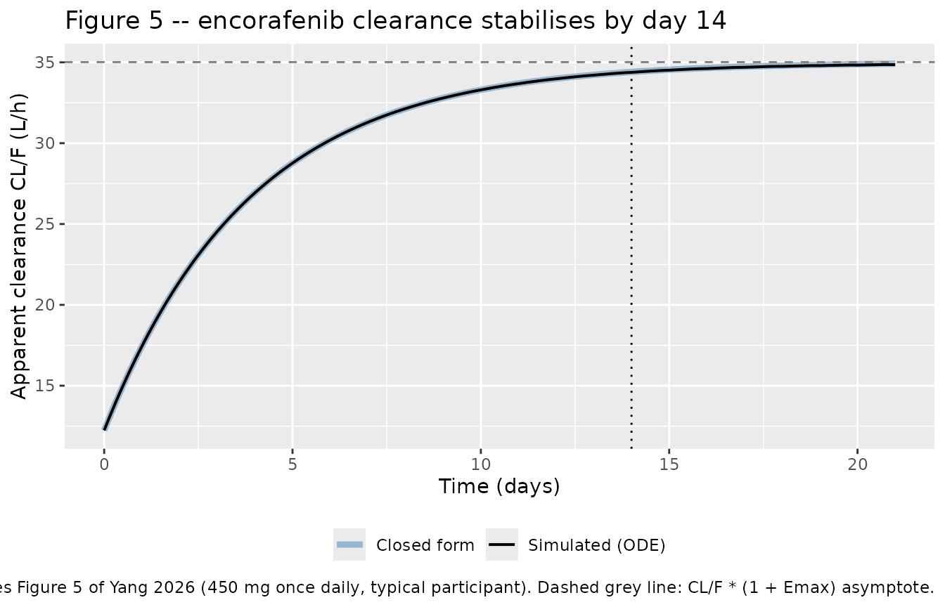
pick <- function(day) sim_typ$cl[which.min(abs(sim_typ$time - day * 24))]
cl_day7  <- pick(7)
cl_day14 <- pick(14)

# Time at which clearance crosses the midpoint of its rise; for the closed-form
# step response this is exactly the published turnover half-life of 64.279 h.
mid <- (cl_day1 + cl_ss_max) / 2
t_half_induction <- approx(x = sim_typ$cl, y = sim_typ$time, xout = mid)$y

max_pct_vs_closed <- max(abs(100 * (sim_typ$cl - sim_typ$cl_closed_form) /
                               sim_typ$cl_closed_form))

fig5 <- tibble::tibble(
  Quantity = c("CL/F at t = 0 (L/h)", "CL/F on day 7 (L/h)", "CL/F on day 14 (L/h)",
               "CL/F plateau (L/h)", "Induction half-life (h)"),
  Simulated = c(sim_typ$cl[1], cl_day7, cl_day14, max(sim_typ$cl), t_half_induction),
  `Yang 2026` = c(12.2, NA, NA, 35.0, 64.3),
  Source = c("Results 3.3 / Table 2", "Figure 5 (reads about 31.3)",
             "Figure 5 (reads about 34.4)", "Results 3.3 (186% rise to 35 L/h)",
             "Table 2 turnover half-life")
)
knitr::kable(fig5, digits = 3,
caption = "Typical-value clearance trajectory versus Yang 2026.")| Quantity | Simulated | Yang 2026 | Source |
|---|---|---|---|
| CL/F at t = 0 (L/h) | 12.238 | 12.2 | Results 3.3 / Table 2 |
| CL/F on day 7 (L/h) | 31.291 | NA | Figure 5 (reads about 31.3) |
| CL/F on day 14 (L/h) | 34.382 | NA | Figure 5 (reads about 34.4) |
| CL/F plateau (L/h) | 34.861 | 35.0 | Results 3.3 (186% rise to 35 L/h) |
| Induction half-life (h) | 64.281 | 64.3 | Table 2 turnover half-life |
stopifnot(
  # Deterministic typical-value solve: the ODE must track its own closed form.
  # Realised 0.17%; the small gap is the trough dip of EFF below Emax once
  # Ctrough approaches EC50 late in the course.
  max_pct_vs_closed < 0.5,
  # Fig. 5 read-offs.
  cl_day7  > 30.5 && cl_day7  < 32.0,
  cl_day14 > 33.8 && cl_day14 < 35.0,
  # Plateau within 1% of CL/F * (1 + Emax).
  abs(max(sim_typ$cl) - cl_ss_max) / cl_ss_max < 0.01,
  # Induction half-life recovers the published 64.279 h.
  abs(t_half_induction - 64.279) < 3
)
Replicating the reported covariate effects
Yang 2026 Results 3.4 quantifies the retained covariate effects at the 10th and 90th percentiles of the analysis population. These are pure arithmetic on Eqs. 6 and 7, so they are checked exactly.
tv_cl <- function(age, crc = 0, other = 0) {
  12.238 * (age / 58)^-0.326 * (1 - 0.175 * crc) * (1 - 0.0938 * other)
}
tv_vc <- function(wt) 61.73 * (wt / 76)^0.588

cov_tab <- tibble::tibble(
  Scenario = c("CL/F at age 38 years", "CL/F at age 73 years",
               "Vc/F at 56 kg", "Vc/F at 100 kg",
               "CL/F melanoma vs mCRC (ratio)", "CL/F melanoma vs other tumor (ratio)"),
  Model = c(tv_cl(38), tv_cl(73), tv_vc(56), tv_vc(100),
            tv_cl(58) / tv_cl(58, crc = 1), tv_cl(58) / tv_cl(58, other = 1)),
  `Yang 2026` = c(14.0, 11.3, 51.6, 72.5, NA, NA),
  Units = c("L/h", "L/h", "L", "L", "unitless", "unitless")
)
knitr::kable(cov_tab, digits = 3,
caption = "Covariate effects reproduced from Yang 2026 Results 3.4.")| Scenario | Model | Yang 2026 | Units |
|---|---|---|---|
| CL/F at age 38 years | 14.047 | 14.0 | L/h |
| CL/F at age 73 years | 11.354 | 11.3 | L/h |
| Vc/F at 56 kg | 51.584 | 51.6 | L |
| Vc/F at 100 kg | 72.540 | 72.5 | L |
| CL/F melanoma vs mCRC (ratio) | 1.212 | NA | unitless |
| CL/F melanoma vs other tumor (ratio) | 1.104 | NA | unitless |
Virtual cohort
Individual data are not publicly available, so a virtual cohort is drawn to match the Table 1 marginal distributions: age from N(57.10, 13.48) truncated to 19-94 years, body weight from N(77.79, 18.79) truncated to 34-168 kg. Two arms are simulated, each at 200 participants (the per-arm cap for this package’s validation vignettes):
- melanoma, 450 mg once daily (the approved dose with binimetinib);
- metastatic CRC, 300 mg once daily (the approved dose with cetuximab).
# set.seed() seeds R's RNG (the covariate draws below). It does NOT seed
# rxode2's simulation RNG, whose streams are partitioned per solver thread --
# so the eta draws differ between a 16-thread workstation and a 2-core CI
# runner. Every assertion downstream is written to hold for any cohort this
# model can produce.
set.seed(20260901)

n_arm <- 200

make_cohort <- function(n, dose_mg, crc, other, arm, id_offset = 0L) {
  subj <- tibble::tibble(
    id          = id_offset + seq_len(n),
    arm         = arm,
    dose_mg     = dose_mg,
    AGE         = pmin(94, pmax(19, rnorm(n, 57.10, 13.48))),
    WT          = pmin(168, pmax(34, rnorm(n, 77.79, 18.79))),
    TUMTP_CRC   = crc,
    TUMTP_OTHER = other
  )
  obs_times <- sort(unique(c(
    seq(0, tau, by = 0.25),                                  # first dosing interval
    seq((ndays - 1) * tau, ndays * tau, by = 0.25),          # last (steady-state) interval
    seq(0, ndays * tau, by = 6)                              # coarse grid for the profile plot
  )))
  doses <- subj |>
    tidyr::crossing(time = seq(0, (ndays - 1) * tau, by = tau)) |>
    mutate(amt = dose_mg, evid = 1L, cmt = "depot")
  obs <- subj |>
    tidyr::crossing(time = obs_times) |>
    mutate(amt = NA_real_, evid = 0L, cmt = "central")
  bind_rows(doses, obs) |> arrange(id, time, desc(evid))
}

events <- bind_rows(
  make_cohort(n_arm, 450, crc = 0, other = 0, arm = "Melanoma 450 mg QD", id_offset = 0L),
  make_cohort(n_arm, 300, crc = 1, other = 0, arm = "mCRC 300 mg QD",     id_offset = 1000L)
)
stopifnot(!anyDuplicated(unique(events[, c("id", "time", "evid")])))
Simulation
sim <- rxode2::rxSolve(
  mod, events = events,
  keep = c("arm", "dose_mg", "AGE", "WT")
) |>
  as.data.frame() |>
  filter(!is.na(Cc))
#> ℹ parameter labels from comments will be replaced by 'label()'

stopifnot(nrow(sim) > 0, all(sim$Cc >= 0))
# Companion to Figure 2 of Yang 2026 (observed concentration versus time by
# study and dose level): the simulated median with a 5th-95th percentile band.
sim |>
  filter(time %% 6 == 0, time > 0) |>   # drop the pre-dose zero: it has no log scale
  group_by(arm, time) |>
  summarise(Q05 = quantile(Cc, 0.05), Q50 = median(Cc), Q95 = quantile(Cc, 0.95),
            .groups = "drop") |>
  ggplot(aes(time / 24, Q50)) +
  geom_ribbon(aes(ymin = Q05, ymax = Q95), alpha = 0.25) +
  geom_line() +
  facet_wrap(~arm) +
  scale_y_log10() +
  labs(x = "Time (days)", y = "Encorafenib concentration (ng/mL)",
       title = "Simulated concentration-time profiles (median, 5th-95th percentile)",
       caption = "Companion to Figure 2 of Yang 2026; the drop after day 1 is net autoinduction.")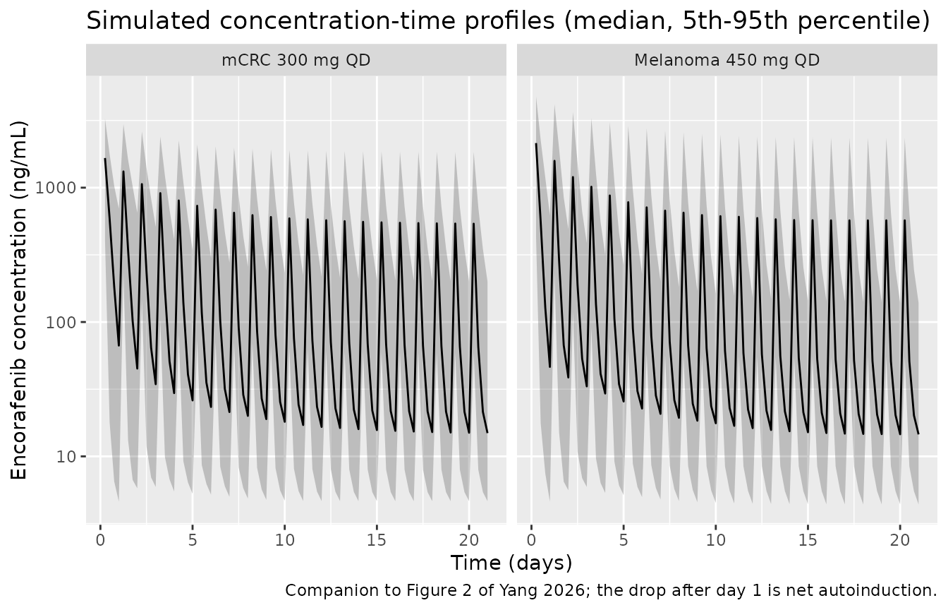
sim |>
  filter(time %% 6 == 0) |>
  group_by(arm, time) |>
  summarise(Q50 = median(cl), Q05 = quantile(cl, 0.05), Q95 = quantile(cl, 0.95),
            .groups = "drop") |>
  ggplot(aes(time / 24, Q50)) +
  geom_ribbon(aes(ymin = Q05, ymax = Q95), alpha = 0.25) +
  geom_line() +
  geom_vline(xintercept = 14, linetype = "dotted") +
  facet_wrap(~arm) +
  labs(x = "Time (days)", y = "Apparent clearance CL/F (L/h)",
       title = "Individual clearance trajectories under autoinduction",
       caption = "Cohort version of Figure 5 of Yang 2026; dotted line marks day 14.")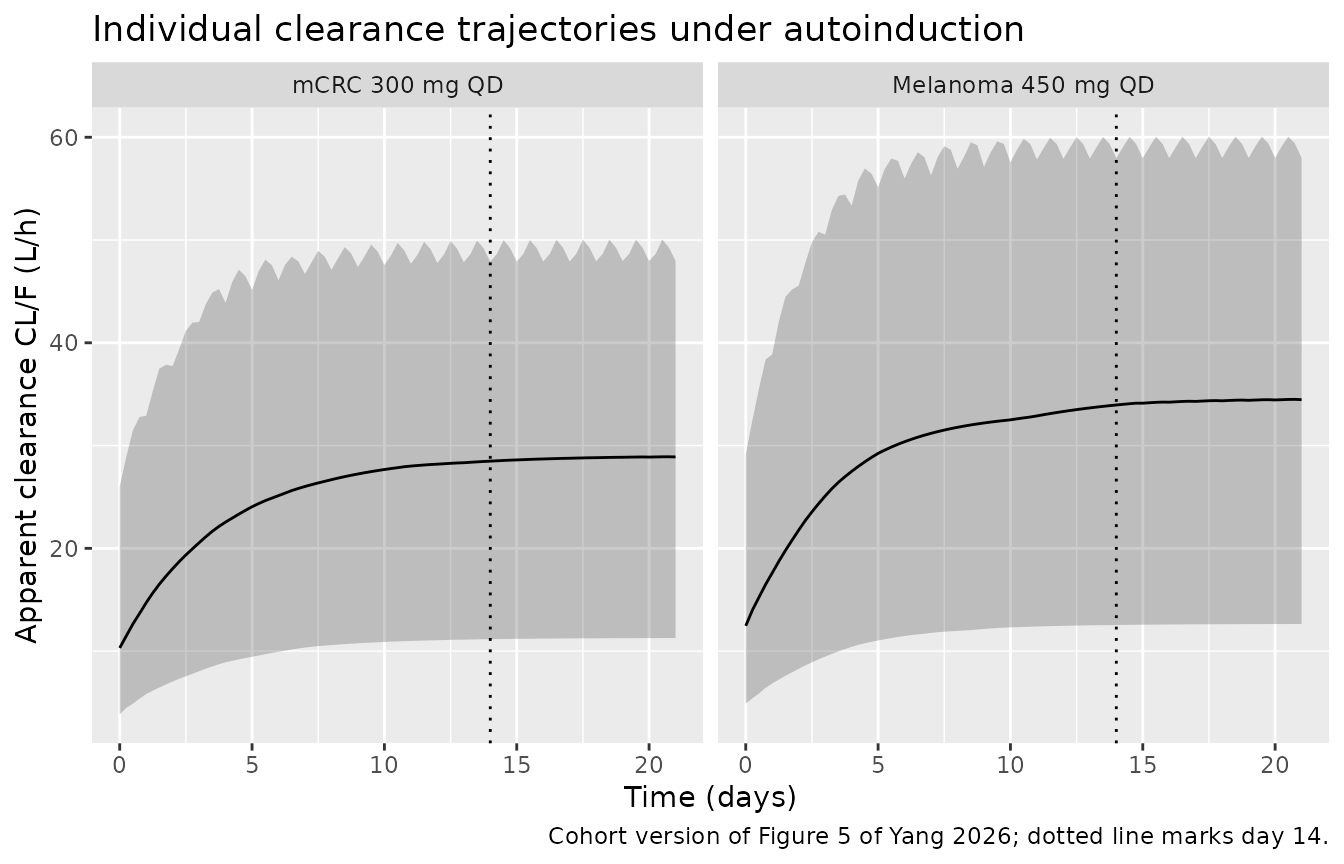
PKNCA validation
NCA is run over two intervals per participant: the first dosing interval (0-24 h, pre-induction) and the final dosing interval at steady state (480-504 h, day 20 to day 21, by which point the enzyme pool has reached more than 99% of its asymptote).
sim_nca <- sim |> select(id, time, Cc, arm)

# Guarantee a pre-dose row per (id, arm); Cc = 0 is correct for an
# extravascular model.
sim_nca <- bind_rows(
  sim_nca,
  sim_nca |> distinct(id, arm) |> mutate(time = 0, Cc = 0)
) |>
  distinct(id, arm, time, .keep_all = TRUE) |>
  arrange(id, time)

conc_obj <- PKNCA::PKNCAconc(sim_nca, Cc ~ time | arm + id,
                             concu = "ng/mL", timeu = "h")

dose_df <- events |>
  filter(evid == 1) |>
  select(id, time, amt, arm)
dose_obj <- PKNCA::PKNCAdose(as.data.frame(dose_df), amt ~ time | arm + id,
                             doseu = "mg")

intervals <- data.frame(
  start   = c(0, (ndays - 1) * tau),
  end     = c(tau, ndays * tau),
  cmax    = TRUE,
  tmax    = TRUE,
  cmin    = TRUE,
  auclast = TRUE,
  cav     = TRUE
)

nca_res <- suppressWarnings(
  PKNCA::pk.nca(PKNCA::PKNCAdata(conc_obj, dose_obj, intervals = intervals))
)

nca_wide <- as.data.frame(nca_res$result) |>
  filter(PPTESTCD %in% c("cmax", "tmax", "cmin", "auclast", "cav")) |>
  tidyr::pivot_wider(id_cols = c(arm, id, start, end),
                     names_from = PPTESTCD, values_from = PPORRES) |>
  mutate(Interval = ifelse(start == 0, "Day 1 (0-24 h)", "Steady state (480-504 h)"))

nca_wide |>
  group_by(arm, Interval) |>
  summarise(cmax = median(cmax), tmax = median(tmax), cmin = median(cmin),
            auclast = median(auclast), cav = median(cav), .groups = "drop") |>
  rename(
    "Arm"                    = arm,
    "Cmax (ng/mL)"           = cmax,
    "Tmax (h)"               = tmax,
    "Cmin (ng/mL)"           = cmin,
    "AUC0-tau (ng*h/mL)"     = auclast,
    "Cavg (ng/mL)"           = cav
  ) |>
  knitr::kable(digits = c(0, 0, 1, 2, 1, 0, 1),
caption = "Median simulated NCA parameters by arm and interval.")| Arm | Interval | Cmax (ng/mL) | Tmax (h) | Cmin (ng/mL) | AUC0-tau (ng*h/mL) | Cavg (ng/mL) |
|---|---|---|---|---|---|---|
| Melanoma 450 mg QD | Day 1 (0-24 h) | 4598.9 | 2.00 | 0.0 | 30791 | 1283.0 |
| Melanoma 450 mg QD | Steady state (480-504 h) | 3260.0 | 1.25 | 14.6 | 13017 | 542.4 |
| mCRC 300 mg QD | Day 1 (0-24 h) | 3202.1 | 2.00 | 0.0 | 23602 | 983.4 |
| mCRC 300 mg QD | Steady state (480-504 h) | 2451.1 | 1.50 | 14.9 | 10356 | 431.5 |
Cmin over the first interval is 0 by construction: the
interval starts at the pre-dose sample, where the concentration is zero
for an extravascular first dose. Only the steady-state Cmin
is a trough in the usual sense.
Yang 2026 reports no NCA table of its own, so there is nothing to
feed nlmixr2lib::ncaComparisonTable(). The NCA output is
instead used for two model-implied identities and one published
claim.
d1 <- nca_wide |> filter(start == 0) |>
  select(arm, id, auc_day1 = auclast, cmax_day1 = cmax)
ss <- nca_wide |> filter(start == (ndays - 1) * tau) |>
  select(arm, id, auc_ss = auclast, cmax_ss = cmax)

# Model clearance at the end of the final dosing interval, per subject.
cl_end <- sim |> filter(time == ndays * tau) |> select(id, cl_model = cl)

chk <- d1 |>
  inner_join(ss, by = c("arm", "id")) |>
  inner_join(cl_end, by = "id") |>
  inner_join(distinct(events, id, dose_mg), by = "id") |>
  mutate(
    accum_ratio = auc_ss / auc_day1,
    # AUC0-tau is in ng*h/mL; 1 ng/mL = 1e-3 mg/L, so CL (L/h) = 1000 * dose / AUC.
    cl_from_nca = 1000 * dose_mg / auc_ss,
    pct_diff    = 100 * (cl_from_nca - cl_model) / cl_model
  )

chk_summary <- chk |>
  group_by(arm) |>
  summarise(
    `Median AUC0-tau SS / AUC0-tau day 1` = median(accum_ratio),
    `Median CL from dose/AUC (L/h)`       = median(cl_from_nca),
    `Median model CL at 504 h (L/h)`      = median(cl_model),
    `Median absolute difference (%)`      = median(abs(pct_diff)),
    `90th percentile absolute difference (%)` = quantile(abs(pct_diff), 0.9),
    .groups = "drop"
  ) |>
  rename("Arm" = arm)
knitr::kable(chk_summary, digits = 3,
caption = "Dose/AUC0-tau at steady state versus the model's own clearance.")| Arm | Median AUC0-tau SS / AUC0-tau day 1 | Median CL from dose/AUC (L/h) | Median model CL at 504 h (L/h) | Median absolute difference (%) | 90th percentile absolute difference (%) |
|---|---|---|---|---|---|
| Melanoma 450 mg QD | 0.452 | 34.571 | 34.467 | 0.331 | 1.616 |
| mCRC 300 mg QD | 0.474 | 28.968 | 28.893 | 0.250 | 1.808 |
cv_cl_day1 <- sim |>
  filter(time == 0) |>
  summarise(cv = 100 * sd(cl) / mean(cl)) |>
  pull(cv)
signif(cv_cl_day1, 4)
#> [1] 59.21

stopifnot(
  # Identity: at steady state, dose / AUC0-tau recovers the model's own
  # clearance. Not exact, because clearance varies slightly within the
  # interval as Ctrough approaches EC50, so this is asserted on the centre
  # and on a robust quantile rather than on the extreme (realised medians
  # 0.33% / 0.24%, 90th percentiles 1.6% / 1.8%).
  all(chk_summary$`Median absolute difference (%)` < 3),
  all(chk_summary$`90th percentile absolute difference (%)` < 6),
  # Yang 2026 Introduction (from the product label): steady-state exposure is
  # about 50% lower than after the first dose. Realised medians 0.45 / 0.47.
  all(chk_summary$`Median AUC0-tau SS / AUC0-tau day 1` > 0.30),
  all(chk_summary$`Median AUC0-tau SS / AUC0-tau day 1` < 0.70),
  # Day-1 clearance spread: the 56.48% CV IIV on CL/F plus the age covariate
  # spread. Realised about 59%.
  cv_cl_day1 > 40, cv_cl_day1 < 85
)
The model reproduces the paper’s central quantitative claim about net autoinduction: steady-state exposure over a dosing interval is roughly half of the first-dose exposure, and the dose/AUC0-tau clearance at steady state agrees with the model’s own time-varying clearance to well under a percent at the median.
Assumptions and deviations
-
The residual error is
combined1(), and both of its components take the one published value. Yang 2026 Eq. 5 is typeset asY_ij = F_ij * (1 + W * eps_ij) + W * eps_ijwithsigma^2fixed to 1. The same unsubscriptedWappears in both terms – this was verified against the typeset equation in the PDF, not only against a text extraction, because symbol-font extraction routinely drops subscripts. Collecting the singleeps_ijgives a residual standard deviation ofW * (1 + F_ij), a linear sum of an additive and a proportional term. In nlmixr2 that isadd(addSd) + prop(propSd) + combined1(), and it is not the same asadd() + prop()on its own, which draws two independent epsilons and combines them in quadrature (W * sqrt(1 + F^2)). Table 2 publishes one error theta (theta_Prop err= 0.589), which isW, so both components are set to that value and nothing is invented. Two caveats are recorded here rather than silently resolved: the Methods sentence introducing Eq. 5 calls it “a proportional model”, and the following sentence saysW“was estimated as two of the thetas”. If the authors did in fact estimate two distinct thetas, only one of them is published anywhere in the article or in the online supplement (which contains Table S1 and Figures S1-S5 only, no parameter values). The printed equation is followed, per the standing rule that an equation outranks narrative text. Practically the choice only matters below about 50 ng/mL: an additive standard deviation of 0.589 ng/mL sits at the floor of the observed concentration range in Yang 2026 Fig. 2, which extends down to about 1 ng/mL. -
The narrative percentages for tumor type restate the
coefficients, not the ratios. Results 3.4 says melanoma CL/F is
“approximately 17.5% higher than in those with metastatic CRC” and
“approximately 9% higher” than in the other tumor group. Those are the
magnitudes of the Eq. 6 coefficients, which lower CL/F in the
non-reference groups; the implied melanoma-to-mCRC ratio is
1 / (1 - 0.175)= 1.212 (21.2% higher) and the melanoma-to-other ratio is1 / (1 - 0.0938)= 1.104 (10.4% higher). The model encodes the coefficients as printed in Eq. 6 and Table 2; the covariate table above reports both ratios so the difference is visible. -
e_tumtp_other_cluses the equation’s precision. Eq. 6 prints -0.0938; Table 2 rounds the same theta to -0.094. The equation value is used. -
The enzyme turnover parameter is entered as
kENZ, not as the half-life. Table 2 reportstheta_Turnover HL= 64.279 h with an IIV of 15.81% CV; the model storeslkenz = log(log(2) / 64.279)= log(0.010784) withetalkenz ~ fixed(0.025). On the log scale an eta onkENZis exactly the negative of an eta on the half-life with the same variance, so the two encodings are distributionally identical. This follows the enzyme-pool idiom already used bymodellib("Smythe_2012_rifampicin")andmodellib("Clewe_2015_rifampicin"), and reproduces theK_ENZ= 0.0108 /h printed in Results 3.3. -
IIV variances follow the paper’s own %CV
definition. Eq. 4 defines the reported %CV as
sqrt(omega^2) * 100, soomega^2 = (CV / 100)^2rather than the more usuallog(1 + CV^2). This is confirmed internally: the 15.81% CV entries correspond toomega^2= 0.025, exactly the small positive variance that Methods 2.2 says was assigned to random effects estimated near zero under SAEM-IMP with mu-referencing. -
The Hill exponent is fixed with an IIV retained.
Table 2 gives
theta_Gamma= 10 with no RSE, no confidence interval and no bootstrap interval (so it is encoded asfixed()), but also lists a 15.81% CV IIV on it. Both are replicated as published rather than simplified away. Withgamma= 10 the induction driver behaves almost as a switch atEC50= 9.097 ng/mL, which is why the simulated clearance tracks the closed-form step response so closely at clinical doses. -
Concentration units. Amounts are in mg and
Vc/Fis in L, so the model applies an explicit factor of 1000 inCc <- 1000 * central / vcto put the observation on the ng/mL scale used byEC50and by the paper’s figures. -
Screened but unretained covariates are documented, not
modelled. Sex, albumin, total protein, bilirubin, AST, LDH,
eGFR, ECOG performance status and concomitant moderate/strong CYP3A
inhibitor use were all tested and not retained; ALT was not tested
because of its correlation with AST (>0.6), race was not tested
because 90% of participants were White, and concomitant CYP3A
inducer was not tested because 99% of participants had absent
or only weak inducer use. These are recorded in the model file’s
covariatesDataExcludedlist so the provenance of the covariate screen survives, without declaring covariates the model body never references. - The virtual cohort’s covariate distributions are an assumption. Table 1 reports only means, standard deviations, medians and interquartile ranges, so age and weight are drawn from normal distributions matched to the reported mean and SD and truncated to the reported ranges. The paper’s actual distributions (Supplementary Fig. S5) are right-skewed for several laboratory covariates, but none of those enter the final model.
-
Food effect is not modelled. Yang 2026 states this
as a limitation of the analysis itself: fed/fasted status was not
consistently collected across the nine studies, so
Kacarries a fixed 50% IIV rather than an estimated one and no food covariate exists to encode. - Combination partners are not modelled. Binimetinib and cetuximab co-administration were tested as a treatment-type covariate on CL/F and not retained, so the model describes encorafenib disposition irrespective of the combination partner.