Rifampicin (Bilal 2024)
Source:vignettes/articles/Bilal_2024_rifampicin.Rmd
Bilal_2024_rifampicin.RmdModel and source
- Citation: Bilal M, Ullah S, Jaehde U, Trueck C, Zaremba D, Wachall B, Wargenau M, Scheidel B, Wiesen MHJ, Gazzaz M, Chen C, Buesker S, Fuhr U, Taubert M, Dokos C. Assessment of body mass-related covariates for rifampicin pharmacokinetics in healthy Caucasian volunteers. Eur J Clin Pharmacol. 2024;80(9):1271-1283. doi:10.1007/s00228-024-03697-3. Parameter estimates from Table 3 (FFM covariate model column); the structural model and random-effect structure from the Monolix code of the base model in the supplementary material. Fat-free mass follows Janmahasatian et al. (2005) Clin Pharmacokinet 44(10):1051-1065 doi:10.2165/00003088-200544100-00004.
- Article: https://doi.org/10.1007/s00228-024-03697-3
Bilal 2024 analysed rich plasma rifampicin data from a two-period bioequivalence crossover in 24 healthy Caucasian volunteers, each given a single 600 mg oral tablet per period. The structural model is one compartment with a zero-order input after a lag time and Michaelis-Menten elimination (Figure 1, Table 2). The paper’s question was which body-size descriptor best explains the between-subject variability. It reports two final covariate models side by side in Table 3, both bootstrapped. The library ships both:
-
Bilal_2024_rifampicin_ffm: fat-free mass (FFM) on V/F (exponent 1) and Vmax/F (exponent 0.75). This was the best model, with an OFV drop of 56.4 from the base model. -
Bilal_2024_rifampicin_sexwt: male sex on V/F and Vmax/F plus body weight on V/F (exponent 1). This was the second-best model, with an OFV drop of 51.2.
The base model (no covariates) is not shipped as a separate model. Its Table 3 estimates appear in the source trace below.
- FFM model: One-compartment population PK model for a single 600 mg oral dose of rifampicin in healthy Caucasian adult volunteers (Bilal 2024), the fat-free-mass (FFM) covariate model that the authors ranked best. Absorption is a zero-order input of duration Tk0 (0.470 h) into the central compartment after a lag time (0.340 h); elimination is Michaelis-Menten (Vmax/F 190 mg/h, Km 20.1 mg/L) from a central volume V/F of 36.2 L. FFM scales V/F linearly and Vmax/F with a fixed 0.75 exponent, both normalised to the cohort mean FFM of about 50.1 kg. Between-subject variability is on Vmax/F only (18.5%); inter-occasion variability over the two crossover periods is on lag time, Tk0, V/F and Vmax/F, with correlated lag-time and Tk0 occasion effects. Residual error is the Monolix combined1 form (additive 0.060 mg/L plus 11.0% proportional, summed as standard deviations). Dose records into central must carry rate = -2 so the modelled zero-order duration applies.
- Sex + BW model: One-compartment population PK model for a single 600 mg oral dose of rifampicin in healthy Caucasian adult volunteers (Bilal 2024), the alternative sex + body weight covariate model that the authors ranked second-best. Absorption is a zero-order input of duration Tk0 (0.470 h) into the central compartment after a lag time (0.340 h); elimination is Michaelis-Menten (Vmax/F 157 mg/h in females, Km 20.2 mg/L) from a central volume V/F of 33.2 L in females. Male sex multiplies V/F by exp(0.190) and Vmax/F by exp(0.420); body weight scales V/F linearly (exponent fixed to 1), normalised to the cohort mean weight of about 72.6 kg. Between-subject variability is on Vmax/F only (19.7%); inter-occasion variability over the two crossover periods is on lag time, Tk0, V/F and Vmax/F, with correlated lag-time and Tk0 occasion effects. Residual error is the Monolix combined1 form (additive 0.060 mg/L plus 11.0% proportional, summed as standard deviations). Dose records into central must carry rate = -2 so the modelled zero-order duration applies.
Population
Twenty-four healthy Caucasian adults (11 men, 13 women) completed the study (EudraCT 2017-004418-24, Cologne, Germany). Table 1 reports the following medians and ranges by sex:
| Female (n = 13) | Male (n = 11) | |
|---|---|---|
| Body weight (kg) | 63.8 (48.5-73.1) | 82.9 (57.8-91.0) |
| Body height (m) | 1.65 (1.55-1.76) | 1.81 (1.63-1.89) |
| FFM (kg) | 39.2 (33.7-44.8) | 63 (47.09-68.9) |
| BMI (kg/m^2) | 23.09 (18.7-26.7) | 24.7 (20.1-29.7) |
| Age (years) | 37.0 (21.0-58.0) | 43.0 (22.0-64.0) |
| BSA (m^2) | 1.66 (1.47-1.85) | 2.05 (1.62-2.18) |
The overall median age was 39.5 years and the overall median weight was 68 kg. Plasma was sampled 19 times after each dose, up to 24 h. That gives 912 concentrations, of which 10.8% were below the 0.1 mg/L LLOQ. The two tablets were bioequivalent and had no effect on any parameter, so both periods were pooled and treated as two occasions.
Source trace
| Element | Source | Value (FFM model / sex + BW model / base model) |
|---|---|---|
| One compartment, zero-order input after a lag, Michaelis-Menten elimination | Figure 1; Table 2 model 1; supplementary Monolix code
pkmodel(Tlag, Tk0, V, Vm, Km)
|
– |
ltlag (Tlag, h) |
Table 3 | 0.340 / 0.340 / 0.340 |
ld1 (Tk0, h) |
Table 3 | 0.470 / 0.470 / 0.460 |
lvc (V/F, L) |
Table 3 | 36.2 / 33.2 (female) / 36.2 |
lvmax (Vmax/F, mg/h) |
Table 3 | 190 / 157 (female) / 191 |
lkm (Km, mg/L) |
Table 3 | 20.1 / 20.2 / 20.4 |
e_ffm_vc, e_ffm_vmax
|
Table 3, both fixed | 1, 0.75 / – / – |
e_wt_vc |
Table 3, fixed | – / 1 / – |
e_sexm_vc, e_sexm_vmax
|
Table 3 | – / 0.190, 0.420 / – |
Covariate form PK_pop * (COV / weighted mean)^beta
|
Eq. 1 | – |
| FFM, Janmahasatian with BMI | Eqs. 2-3 | – |
etalvmax (IIV Vmax/F, omega) |
Table 3 | 0.185 / 0.197 / 0.390 |
| IIV V/F | Table 3 | none / none / 0.244 |
etaiov_tlag_* (IOV Tlag) |
Table 3 | 0.390 / 0.388 / 0.391 |
etaiov_d1_* (IOV Tk0) |
Table 3 | 0.655 / 0.657 / 0.669 |
| Correlation of IOV Tlag and IOV Tk0 | Table 3; Monolix
correlation = {level=id*occ, r(Tlag, Tk0)}
|
0.410 / 0.420 / 0.390 |
etaiov_vc_* (IOV V/F) |
Table 3 | 0.149 / 0.154 / 0.135 |
etaiov_vmax_* (IOV Vmax/F) |
Table 3 | 0.0939 / 0.0932 / 0.0938 |
addSd (mg/L), propSd
|
Table 3; Monolix errorModel=combined1(a, b)
|
0.060, 0.110 / 0.060, 0.110 / 0.061, 0.110 |
| FFM reference 50.1 kg, WT reference 72.6 kg | Derived from Table 1 (see Assumptions) | – |
Virtual cohort
The cohort mirrors the study’s 13:11 female-to-male split, with 200 subjects in total. Height and BMI are drawn per sex around the Table 1 medians and truncated to the Table 1 ranges. Body weight is then BMI x height^2, and FFM follows from the paper’s Eqs. 2-3.
ffm_janmahasatian <- function(wt, bmi, sexf) {
  ifelse(sexf == 1, 9270 * wt / (8780 + 244 * bmi), 9270 * wt / (6680 + 216 * bmi))
}
rtrunc <- function(n, mean, sd, lo, hi) {
  pmin(pmax(rnorm(n, mean, sd), lo), hi)
}

set.seed(20240509)
n_f <- 108
n_m <- 92
cohort <- tibble(
  id = seq_len(n_f + n_m),
  SEXF = c(rep(1, n_f), rep(0, n_m)),
  BMI = c(rtrunc(n_f, 23.09, 2, 18.7, 26.7), rtrunc(n_m, 24.7, 2.4, 20.1, 29.7)),
  HT_m = c(rtrunc(n_f, 1.65, 0.055, 1.55, 1.76), rtrunc(n_m, 1.81, 0.065, 1.63, 1.89))
) |>
  mutate(
    WT = BMI * HT_m^2,
    FFM = ffm_janmahasatian(WT, BMI, SEXF),
    sex = ifelse(SEXF == 1, "female", "male")
  )

cohort |>
  group_by(sex) |>
  summarise(
    n = n(),
    WT = sprintf("%.1f (%.1f-%.1f)", median(WT), min(WT), max(WT)),
    FFM = sprintf("%.1f (%.1f-%.1f)", median(FFM), min(FFM), max(FFM)),
    BMI = sprintf("%.1f (%.1f-%.1f)", median(BMI), min(BMI), max(BMI))
  ) |>
knitr::kable(caption = "Virtual cohort, median (range).")| sex | n | WT | FFM | BMI |
|---|---|---|---|---|
| female | 108 | 63.6 (45.0-82.7) | 40.6 (31.3-50.1) | 23.2 (18.7-26.7) |
| male | 92 | 80.4 (66.3-104.3) | 61.6 (52.4-74.5) | 25.1 (20.2-29.7) |
Simulation
Each subject receives one 600 mg dose into central with
rate = -2. The -2 tells rxode2 to use the
modelled zero-order duration Tk0, and OCC = 1 selects the
first-period occasion effects. The paper’s 19 sampling times are kept,
and observations every 0.25 h out to 48 h are added for NCA.
obs_times <- sort(unique(c(
  0, 0.16, 0.33, 0.5, 0.75, 1, 1.25, 1.5, 1.75, 2, 2.25, 2.5, 3, 3.5, 4,
  6, 9, 12, 16, 24, seq(0, 48, by = 0.25)
)))
make_events <- function(cov) {
  dose <- cov |> mutate(time = 0, amt = 600, rate = -2, evid = 1, cmt = "central")
  obs <- tidyr::expand_grid(cov, time = obs_times) |>
    mutate(amt = 0, rate = 0, evid = 0, cmt = "central")
  bind_rows(dose, obs) |>
    mutate(OCC = 1) |>
    arrange(id, time, desc(evid))
}
events <- make_events(cohort)

mod_ffm <- readModelDb("Bilal_2024_rifampicin_ffm")
mod_sexwt <- readModelDb("Bilal_2024_rifampicin_sexwt")

rxode2::rxSetSeed(20240509)
sim_ffm <- rxode2::rxSolve(mod_ffm, events, keep = "sex", returnType = "data.frame")
#> ℹ parameter labels from comments will be replaced by 'label()'
#> Warning: some etas defaulted to non-mu referenced, possible parsing error: etaiov_tlag_1, etaiov_d1_1, etaiov_tlag_2, etaiov_d1_2, etaiov_vc_1, etaiov_vc_2, etaiov_vmax_1, etaiov_vmax_2
#> as a work-around try putting the mu-referenced expression on a simple line
sim_sexwt <- rxode2::rxSolve(mod_sexwt, events, keep = "sex", returnType = "data.frame")
#> ℹ parameter labels from comments will be replaced by 'label()'
#> Warning: some etas defaulted to non-mu referenced, possible parsing error: etaiov_tlag_1, etaiov_d1_1, etaiov_tlag_2, etaiov_d1_2, etaiov_vc_1, etaiov_vc_2, etaiov_vmax_1, etaiov_vmax_2
#> as a work-around try putting the mu-referenced expression on a simple line
pred_ffm <- rxode2::rxSolve(rxode2::zeroRe(mod_ffm), events, returnType = "data.frame")
#> ℹ parameter labels from comments will be replaced by 'label()'
#> Warning: some etas defaulted to non-mu referenced, possible parsing error: etaiov_tlag_1, etaiov_d1_1, etaiov_tlag_2, etaiov_d1_2, etaiov_vc_1, etaiov_vc_2, etaiov_vmax_1, etaiov_vmax_2
#> as a work-around try putting the mu-referenced expression on a simple line
#> Warning: some etas defaulted to non-mu referenced, possible parsing error: etaiov_tlag_1, etaiov_d1_1, etaiov_tlag_2, etaiov_d1_2, etaiov_vc_1, etaiov_vc_2, etaiov_vmax_1, etaiov_vmax_2
#> as a work-around try putting the mu-referenced expression on a simple line
#> ℹ omega/sigma items treated as zero: 'etalvmax', 'etaiov_tlag_1', 'etaiov_d1_1', 'etaiov_tlag_2', 'etaiov_d1_2', 'etaiov_vc_1', 'etaiov_vc_2', 'etaiov_vmax_1', 'etaiov_vmax_2'
#> Warning: multi-subject simulation without without 'omega'
pred_sexwt <- rxode2::rxSolve(rxode2::zeroRe(mod_sexwt), events, returnType = "data.frame")
#> ℹ parameter labels from comments will be replaced by 'label()'
#> Warning: some etas defaulted to non-mu referenced, possible parsing error: etaiov_tlag_1, etaiov_d1_1, etaiov_tlag_2, etaiov_d1_2, etaiov_vc_1, etaiov_vc_2, etaiov_vmax_1, etaiov_vmax_2
#> as a work-around try putting the mu-referenced expression on a simple line
#> Warning: some etas defaulted to non-mu referenced, possible parsing error: etaiov_tlag_1, etaiov_d1_1, etaiov_tlag_2, etaiov_d1_2, etaiov_vc_1, etaiov_vc_2, etaiov_vmax_1, etaiov_vmax_2
#> as a work-around try putting the mu-referenced expression on a simple line
#> ℹ omega/sigma items treated as zero: 'etalvmax', 'etaiov_tlag_1', 'etaiov_d1_1', 'etaiov_tlag_2', 'etaiov_d1_2', 'etaiov_vc_1', 'etaiov_vc_2', 'etaiov_vmax_1', 'etaiov_vmax_2'
#> Warning: multi-subject simulation without without 'omega'
Replicate published figures
Figure 6: prediction-corrected VPC
Figure 6 shows the prediction-corrected VPC for each covariate model. The 10th, 50th and 90th percentiles of the simulated data (dotted lines) were read from the figure by the maintainers, to about 0.5 mg/L. The same prediction correction is applied here: each simulated concentration is scaled by the bin median of the typical-value prediction divided by the subject’s own typical-value prediction, and the paper’s sampling times are used as bins.
fig6 <- tibble::tribble(
  ~model, ~time, ~p10, ~p50, ~p90,
  "Sex + BW", 1.5, 11.0, 15.0, 19.0,
  "Sex + BW", 4, 8.6, 10.6, 14.0,
  "Sex + BW", 6, 5.4, 7.6, 10.6,
  "Sex + BW", 9, 2.3, 4.2, 7.0,
  "Sex + BW", 12, 0.8, 2.0, 3.9,
  "Sex + BW", 16, 0.2, 0.7, 1.8,
  "FFM", 1.5, 11.0, 15.0, 19.5,
  "FFM", 4, 8.2, 10.5, 13.0,
  "FFM", 6, 5.0, 7.0, 9.5,
  "FFM", 9, 2.0, 3.9, 6.0,
  "FFM", 12, 0.8, 1.9, 3.8,
  "FFM", 16, 0.2, 0.7, 1.8
)

pc_vpc <- function(sim, pred, label) {
  sim |>
    filter(time %in% fig6$time) |>
    select(id, time, sim) |>
    left_join(pred |> select(id, time, pred = Cc), by = c("id", "time")) |>
    group_by(time) |>
    mutate(pcsim = sim * median(pred) / pred) |>
    summarise(
      sim_p10 = quantile(pcsim, 0.1),
      sim_p50 = median(pcsim),
      sim_p90 = quantile(pcsim, 0.9),
      .groups = "drop"
    ) |>
    mutate(model = label)
}
vpc <- bind_rows(
  pc_vpc(sim_sexwt, pred_sexwt, "Sex + BW"),
  pc_vpc(sim_ffm, pred_ffm, "FFM")
) |>
  left_join(fig6, by = c("model", "time"))

vpc |>
  mutate(across(c(sim_p10:sim_p90, p10:p90), ~ round(.x, 2))) |>
  select(model, time, p10, sim_p10, p50, sim_p50, p90, sim_p90) |>
  dplyr::rename(
    "Model" = model, "Time (h)" = time,
    "P10 Fig. 6" = p10, "P10 sim" = sim_p10,
    "Median Fig. 6" = p50, "Median sim" = sim_p50,
    "P90 Fig. 6" = p90, "P90 sim" = sim_p90
  ) |>
knitr::kable(caption = "Prediction-corrected percentiles, simulation vs Figure 6 (mg/L).")| Model | Time (h) | P10 Fig. 6 | P10 sim | Median Fig. 6 | Median sim | P90 Fig. 6 | P90 sim |
|---|---|---|---|---|---|---|---|
| Sex + BW | 1.5 | 11.0 | 11.66 | 15.0 | 14.96 | 19.0 | 19.25 |
| Sex + BW | 4.0 | 8.6 | 8.32 | 10.6 | 10.95 | 14.0 | 14.13 |
| Sex + BW | 6.0 | 5.4 | 5.11 | 7.6 | 8.05 | 10.6 | 11.08 |
| Sex + BW | 9.0 | 2.3 | 1.96 | 4.2 | 4.59 | 7.0 | 7.29 |
| Sex + BW | 12.0 | 0.8 | 0.67 | 2.0 | 2.02 | 3.9 | 4.43 |
| Sex + BW | 16.0 | 0.2 | 0.12 | 0.7 | 0.71 | 1.8 | 2.00 |
| FFM | 1.5 | 11.0 | 11.59 | 15.0 | 14.87 | 19.5 | 19.71 |
| FFM | 4.0 | 8.2 | 7.77 | 10.5 | 10.19 | 13.0 | 13.20 |
| FFM | 6.0 | 5.0 | 5.05 | 7.0 | 7.22 | 9.5 | 9.89 |
| FFM | 9.0 | 2.0 | 1.96 | 3.9 | 3.92 | 6.0 | 5.91 |
| FFM | 12.0 | 0.8 | 0.74 | 1.9 | 1.79 | 3.8 | 3.78 |
| FFM | 16.0 | 0.2 | 0.20 | 0.7 | 0.74 | 1.8 | 1.91 |
vpc |>
  tidyr::pivot_longer(c(sim_p10, sim_p50, sim_p90), names_to = "pct", values_to = "sim") |>
  ggplot(aes(time, sim, group = pct)) +
  geom_line(colour = "steelblue") +
  geom_point(
    data = tidyr::pivot_longer(fig6, c(p10, p50, p90), names_to = "pct", values_to = "conc"),
    aes(time, conc), colour = "firebrick", inherit.aes = FALSE
  ) +
  facet_wrap(~model) +
  labs(x = "Time after dose (h)", y = "Prediction-corrected rifampicin (mg/L)")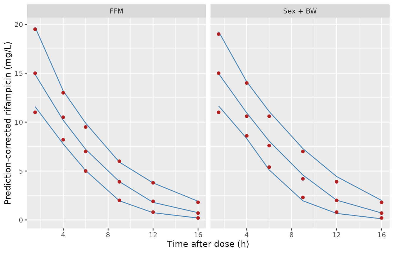
Replicates Figure 6 of Bilal 2024 (prediction-corrected VPC). Lines: simulated 10th, 50th and 90th percentiles; points: the percentiles read from Figure 6.
vpc_chk <- vpc |> mutate(pct_diff = 100 * (sim_p50 - p50) / p50)
stopifnot(
  # A mis-transcribed Vmax, Km or V shifts the whole median curve by tens
  # of percent; the per-time spread includes the precision of reading the
  # figure.
  abs(median(vpc_chk$pct_diff)) < 15,
  quantile(abs(vpc_chk$pct_diff), 0.9) < 30
)
The simulated 10th-90th percentile band also matches Figure 6. Reading the Table 3 random effects as variances instead of standard deviations would roughly double the width of the band at 6-12 h.
Figure 7: AUC against fat-free mass
Figure 7 plots the 5th and 95th percentiles of AUC after a 600 mg dose, simulated with the FFM model at fixed FFM values, against the corresponding percentiles from the base model (dotted lines at about 38 and 232 mg*h/L). The bar ends below were read from the figure by the maintainers. Here 200 subjects are simulated per FFM value.
fig7 <- tibble::tribble(
  ~sex, ~FFM, ~fig_p05, ~fig_p95,
  "female", 30, 42, 260,
  "female", 40, 39, 241,
  "female", 50, 37, 224,
  "female", 60, 36, 215,
  "male", 50, 38, 222,
  "male", 60, 37, 210,
  "male", 70, 37, 207,
  "male", 80, 37, 199
)
f7_cov <- fig7 |>
  select(sex, FFM) |>
  tidyr::expand_grid(rep = 1:200) |>
  mutate(id = row_number())
f7_events <- make_events(f7_cov |> select(id, sex, FFM)) |> filter(time <= 48)
rxode2::rxSetSeed(7)
f7_sim <- rxode2::rxSolve(mod_ffm, f7_events, keep = "sex", returnType = "data.frame")
f7_auc <- f7_sim |>
  group_by(id, sex, FFM) |>
  summarise(auc = sum(diff(time) * (head(Cc, -1) + tail(Cc, -1)) / 2), .groups = "drop") |>
  group_by(sex, FFM) |>
  summarise(sim_p05 = quantile(auc, 0.05), sim_p50 = median(auc), sim_p95 = quantile(auc, 0.95), .groups = "drop") |>
  left_join(fig7, by = c("sex", "FFM"))
f7_auc |>
  mutate(across(starts_with(c("sim", "fig")), ~ round(.x))) |>
  select(sex, FFM, fig_p05, sim_p05, sim_p50, fig_p95, sim_p95) |>
  dplyr::rename(
    "Sex" = sex, "FFM (kg)" = FFM,
    "P5 Fig. 7" = fig_p05, "P5 sim" = sim_p05, "Median sim" = sim_p50,
    "P95 Fig. 7" = fig_p95, "P95 sim" = sim_p95
  ) |>
knitr::kable(caption = "AUC0-48 (mg*h/L) after 600 mg, FFM model, simulation vs Figure 7.")| Sex | FFM (kg) | P5 Fig. 7 | P5 sim | Median sim | P95 Fig. 7 | P95 sim |
|---|---|---|---|---|---|---|
| female | 30 | 42 | 103 | 155 | 260 | 222 |
| female | 40 | 39 | 79 | 115 | 241 | 154 |
| female | 50 | 37 | 64 | 91 | 224 | 128 |
| female | 60 | 36 | 51 | 75 | 215 | 105 |
| male | 50 | 38 | 61 | 88 | 222 | 126 |
| male | 60 | 37 | 52 | 73 | 210 | 103 |
| male | 70 | 37 | 44 | 63 | 207 | 85 |
| male | 80 | 37 | 42 | 56 | 199 | 80 |
The simulated median AUC falls with FFM as Figure 7 describes, from about 155 mgh/L at 30 kg to about 56 mgh/L at 80 kg. The simulated 5th-95th percentile range is, however, much narrower than Figure 7’s bars. Figure 7’s bars are almost as wide as the base-model range and barely depend on FFM, which Table 3 does not support. With IIV on Vmax/F of 18.5% and small IOV on V/F and Vmax/F, the FFM model cannot produce a 5th-95th AUC range of about six-fold at a fixed FFM. The base model reproduced from Table 3 gives about 45-174 mg*h/L, not the figure’s 38-232. Figure 6 does constrain the random effects, and it agrees with the Table 3 values as encoded. Figure 7 is therefore shown for comparison only and is not used as a check; how the authors generated it cannot be recovered from the paper.
Typical profiles by sex
typ_cov <- tibble(
  id = 1:2, sex = c("female", "male"), SEXF = c(1, 0),
  WT = c(63.8, 82.9), FFM = c(39.2, 63)
)
typ_events <- make_events(typ_cov) |> filter(time <= 24)
typ <- bind_rows(
  rxode2::rxSolve(rxode2::zeroRe(mod_ffm), typ_events, keep = "sex", returnType = "data.frame") |> mutate(model = "FFM"),
  rxode2::rxSolve(rxode2::zeroRe(mod_sexwt), typ_events, keep = "sex", returnType = "data.frame") |> mutate(model = "Sex + BW")
)
#> ℹ parameter labels from comments will be replaced by 'label()'
#> Warning: some etas defaulted to non-mu referenced, possible parsing error: etaiov_tlag_1, etaiov_d1_1, etaiov_tlag_2, etaiov_d1_2, etaiov_vc_1, etaiov_vc_2, etaiov_vmax_1, etaiov_vmax_2
#> as a work-around try putting the mu-referenced expression on a simple line
#> Warning: some etas defaulted to non-mu referenced, possible parsing error: etaiov_tlag_1, etaiov_d1_1, etaiov_tlag_2, etaiov_d1_2, etaiov_vc_1, etaiov_vc_2, etaiov_vmax_1, etaiov_vmax_2
#> as a work-around try putting the mu-referenced expression on a simple line
#> ℹ omega/sigma items treated as zero: 'etalvmax', 'etaiov_tlag_1', 'etaiov_d1_1', 'etaiov_tlag_2', 'etaiov_d1_2', 'etaiov_vc_1', 'etaiov_vc_2', 'etaiov_vmax_1', 'etaiov_vmax_2'
#> Warning: multi-subject simulation without without 'omega'
#> ℹ parameter labels from comments will be replaced by 'label()'
#> Warning: some etas defaulted to non-mu referenced, possible parsing error: etaiov_tlag_1, etaiov_d1_1, etaiov_tlag_2, etaiov_d1_2, etaiov_vc_1, etaiov_vc_2, etaiov_vmax_1, etaiov_vmax_2
#> as a work-around try putting the mu-referenced expression on a simple line
#> Warning: some etas defaulted to non-mu referenced, possible parsing error: etaiov_tlag_1, etaiov_d1_1, etaiov_tlag_2, etaiov_d1_2, etaiov_vc_1, etaiov_vc_2, etaiov_vmax_1, etaiov_vmax_2
#> as a work-around try putting the mu-referenced expression on a simple line
#> ℹ omega/sigma items treated as zero: 'etalvmax', 'etaiov_tlag_1', 'etaiov_d1_1', 'etaiov_tlag_2', 'etaiov_d1_2', 'etaiov_vc_1', 'etaiov_vc_2', 'etaiov_vmax_1', 'etaiov_vmax_2'
#> Warning: multi-subject simulation without without 'omega'
ggplot(typ, aes(time, Cc, colour = sex, linetype = model)) +
  geom_line() +
  labs(x = "Time after dose (h)", y = "Rifampicin (mg/L)")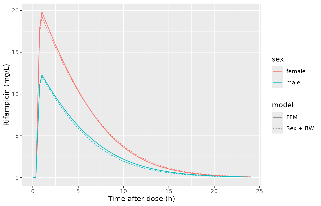
Typical-value rifampicin profiles after 600 mg for a median female and a median male under each covariate model.
PKNCA validation
The paper reports no NCA results; its bioequivalence NCA is “data not shown”. NCA of the simulated cohort is reported per model and sex, which are the groups the paper’s covariate question contrasts.
nca_conc <- bind_rows(
  sim_ffm |> mutate(treatment = paste("FFM", sex)),
  sim_sexwt |> mutate(treatment = paste("Sex + BW", sex))
) |>
  filter(!is.na(Cc)) |>
  select(id, time, Cc, treatment)
nca_dose <- events |>
  filter(evid == 1) |>
  select(id, time, amt, sex) |>
  tidyr::expand_grid(model = c("FFM", "Sex + BW")) |>
  mutate(treatment = paste(model, sex)) |>
  select(id, time, amt, treatment)

conc_obj <- PKNCA::PKNCAconc(nca_conc, Cc ~ time | treatment + id)
dose_obj <- PKNCA::PKNCAdose(nca_dose, amt ~ time | treatment + id)
intervals <- data.frame(
  start = c(0, 0), end = c(Inf, 24),
  cmax = c(TRUE, FALSE), tmax = c(TRUE, FALSE),
  aucinf.obs = c(TRUE, FALSE), half.life = c(TRUE, FALSE),
  auclast = c(FALSE, TRUE)
)
nca_res <- PKNCA::pk.nca(PKNCA::PKNCAdata(conc_obj, dose_obj, intervals = intervals))
nca_summary <- as.data.frame(nca_res$result) |>
  filter(PPTESTCD %in% c("cmax", "tmax", "auclast", "aucinf.obs", "half.life")) |>
  group_by(treatment, PPTESTCD) |>
  summarise(median = median(PPORRES, na.rm = TRUE), .groups = "drop") |>
  tidyr::pivot_wider(names_from = PPTESTCD, values_from = median)
nca_summary |>
  mutate(across(-treatment, ~ signif(.x, 3))) |>
  dplyr::rename(
    "Model and sex" = treatment, "Cmax (mg/L)" = cmax, "Tmax (h)" = tmax,
    "AUC0-24 (mg*h/L)" = auclast, "AUC0-inf (mg*h/L)" = aucinf.obs,
    "t1/2 terminal (h)" = half.life
  ) |>
knitr::kable(caption = "Median simulated NCA parameters after a single 600 mg dose.")| Model and sex | AUC0-inf (mg*h/L) | AUC0-24 (mg*h/L) | Cmax (mg/L) | t1/2 terminal (h) | Tmax (h) |
|---|---|---|---|---|---|
| FFM female | 111.0 | 110.0 | 18.7 | 2.56 | 0.750 |
| FFM male | 72.6 | 71.1 | 12.2 | 2.92 | 1.000 |
| Sex + BW female | 113.0 | 113.0 | 19.1 | 2.65 | 1.000 |
| Sex + BW male | 67.8 | 67.6 | 12.3 | 2.61 | 0.875 |
auc_by <- nca_summary |>
  mutate(model = sub(" (female|male)$", "", treatment), sex = sub("^.* ", "", treatment)) |>
  select(model, sex, aucinf.obs) |>
  tidyr::pivot_wider(names_from = sex, values_from = aucinf.obs) |>
  mutate(ratio_f_m = female / male)
auc_by
#> # A tibble: 2 × 4
#>   model    female  male ratio_f_m
#>   <chr>     <dbl> <dbl>     <dbl>
#> 1 FFM        111.  72.6      1.53
#> 2 Sex + BW   113.  67.8      1.67
stopifnot(
  # The two covariate models were fitted to the same data, so their
  # female/male exposure ratios should agree to within 20%.
  abs(diff(auc_by$ratio_f_m)) / mean(auc_by$ratio_f_m) < 0.2
)
Both models give women a higher exposure than men for the same dose, as the paper concludes. The two models fit the same data, so they should agree on the size of the sex difference, and their female/male AUC ratios agree to within about 9%. The terminal half-life is apparent, because elimination is saturable and the half-life lengthens at higher concentrations.
Form of the sex effect
The paper does not print the sex equation (see Assumptions). The
table below compares typical-value AUC0-inf for a median female (63.8
kg, FFM 39.2 kg) and a median male (82.9 kg, FFM 63 kg). It uses the
shipped log-scale reading exp(beta), the alternative
(1 + beta) reading, and the FFM model as an external
reference.
typ_auc <- function(mod) {
  ev <- make_events(typ_cov) |> filter(time <= 72)
  rxode2::rxSolve(rxode2::zeroRe(mod), ev, keep = "sex", returnType = "data.frame") |>
    group_by(sex) |>
    summarise(auc = sum(diff(time) * (head(Cc, -1) + tail(Cc, -1)) / 2), .groups = "drop")
}
mod_sexwt_linear <- rxode2::rxode2(mod_sexwt) |>
  rxode2::ini(e_sexm_vc = log(1.19), e_sexm_vmax = log(1.42))
#> ℹ parameter labels from comments will be replaced by 'label()'
#> Warning: some etas defaulted to non-mu referenced, possible parsing error: etaiov_tlag_1, etaiov_d1_1, etaiov_tlag_2, etaiov_d1_2, etaiov_vc_1, etaiov_vc_2, etaiov_vmax_1, etaiov_vmax_2
#> as a work-around try putting the mu-referenced expression on a simple line
#> ℹ change initial estimate of `e_sexm_vc` to `0.173953307123438`
#> ℹ change initial estimate of `e_sexm_vmax` to `0.350656871613169`
sex_reading <- bind_rows(
  typ_auc(mod_sexwt) |> mutate(model = "Sex + BW, exp(beta) (shipped)"),
  typ_auc(mod_sexwt_linear) |> mutate(model = "Sex + BW, 1 + beta"),
  typ_auc(mod_ffm) |> mutate(model = "FFM")
) |>
  tidyr::pivot_wider(names_from = sex, values_from = auc) |>
  mutate(ratio = female / male)
#> ℹ parameter labels from comments will be replaced by 'label()'
#> Warning: some etas defaulted to non-mu referenced, possible parsing error: etaiov_tlag_1, etaiov_d1_1, etaiov_tlag_2, etaiov_d1_2, etaiov_vc_1, etaiov_vc_2, etaiov_vmax_1, etaiov_vmax_2
#> as a work-around try putting the mu-referenced expression on a simple line
#> Warning: some etas defaulted to non-mu referenced, possible parsing error: etaiov_tlag_1, etaiov_d1_1, etaiov_tlag_2, etaiov_d1_2, etaiov_vc_1, etaiov_vc_2, etaiov_vmax_1, etaiov_vmax_2
#> as a work-around try putting the mu-referenced expression on a simple line
#> ℹ omega/sigma items treated as zero: 'etalvmax', 'etaiov_tlag_1', 'etaiov_d1_1', 'etaiov_tlag_2', 'etaiov_d1_2', 'etaiov_vc_1', 'etaiov_vc_2', 'etaiov_vmax_1', 'etaiov_vmax_2'
#> Warning: multi-subject simulation without without 'omega'
#> Warning: some etas defaulted to non-mu referenced, possible parsing error: etaiov_tlag_1, etaiov_d1_1, etaiov_tlag_2, etaiov_d1_2, etaiov_vc_1, etaiov_vc_2, etaiov_vmax_1, etaiov_vmax_2
#> as a work-around try putting the mu-referenced expression on a simple line
#> ℹ omega/sigma items treated as zero: 'etalvmax', 'etaiov_tlag_1', 'etaiov_d1_1', 'etaiov_tlag_2', 'etaiov_d1_2', 'etaiov_vc_1', 'etaiov_vc_2', 'etaiov_vmax_1', 'etaiov_vmax_2'
#> Warning: multi-subject simulation without without 'omega'
#> ℹ parameter labels from comments will be replaced by 'label()'
#> Warning: some etas defaulted to non-mu referenced, possible parsing error: etaiov_tlag_1, etaiov_d1_1, etaiov_tlag_2, etaiov_d1_2, etaiov_vc_1, etaiov_vc_2, etaiov_vmax_1, etaiov_vmax_2
#> as a work-around try putting the mu-referenced expression on a simple line
#> Warning: some etas defaulted to non-mu referenced, possible parsing error: etaiov_tlag_1, etaiov_d1_1, etaiov_tlag_2, etaiov_d1_2, etaiov_vc_1, etaiov_vc_2, etaiov_vmax_1, etaiov_vmax_2
#> as a work-around try putting the mu-referenced expression on a simple line
#> ℹ omega/sigma items treated as zero: 'etalvmax', 'etaiov_tlag_1', 'etaiov_d1_1', 'etaiov_tlag_2', 'etaiov_d1_2', 'etaiov_vc_1', 'etaiov_vc_2', 'etaiov_vmax_1', 'etaiov_vmax_2'
#> Warning: multi-subject simulation without without 'omega'
sex_reading |>
  mutate(across(c(female, male), ~ round(.x, 1)), ratio = round(ratio, 3)) |>
  dplyr::rename(
    "Model" = model, "Female AUC0-inf (mg*h/L)" = female,
    "Male AUC0-inf (mg*h/L)" = male, "Female/male ratio" = ratio
  ) |>
knitr::kable(caption = "Typical-value AUC after 600 mg under each reading of the sex effect.")| Model | Female AUC0-inf (mg*h/L) | Male AUC0-inf (mg*h/L) | Female/male ratio |
|---|---|---|---|
| Sex + BW, exp(beta) (shipped) | 115.2 | 66.5 | 1.732 |
| Sex + BW, 1 + beta | 115.2 | 71.6 | 1.608 |
| FFM | 115.1 | 70.3 | 1.637 |
Assumptions and deviations
- Weighted-mean covariate references (not printed). Eq. 1 normalises each continuous covariate to its observation-weighted mean, and the paper does not print those means. Every subject contributed 38 observations (912 / 24, 19 per period), so the weighted mean equals the arithmetic mean, which is also not printed. The maintainers used the sex-composition-weighted average of the per-sex Table 1 medians: FFM (13 x 39.2 + 11 x 63) / 24 = 50.1 kg and body weight (13 x 63.8 + 11 x 82.9) / 24 = 72.6 kg. Two checks support the FFM value. First, the FFM model’s typical female Vmax/F at the female median FFM, 190 x (39.2 / 50.1)^0.75 = 158 mg/h, matches the female-reference Vmax/F of 157 mg/h in the sex + BW model; an exact match would need 50.6 kg. Second, the Figure 6 median curves are reproduced. The weight reference enters V/F linearly, so an error of 1 kg changes the typical V/F by about 1.4%.
-
Form of the sex effect. The paper says sex was
modelled with “a linear model where females were taken as reference” and
prints no equation. The analysis was run in Monolix, and its
continuous-covariate centring (“weighted mean”) is Monolix’s own option.
Monolix enters a categorical covariate on a log-normal parameter
linearly on the log scale,
log(V) = log(V_pop) + beta * male, so the shipped model usesexp(beta). Male V/F is then 1.21 times, and male Vmax/F 1.52 times, the female value. The alternative(1 + beta)reading gives 1.19 and 1.42. Neither reading can be confirmed from the published figures, because the prediction-corrected VPC removes covariate effects. A comparison with the FFM model points mildly the other way. In the “Form of the sex effect” table, the FFM model’s typical female/male AUC ratio lies closer to the(1 + beta)reading than toexp(beta). Likewise, the FFM model’s male/female ratio of typical Vmax/F at the per-sex median FFM, (63 / 39.2)^0.75 = 1.43, is close to 1.42. The two models are separate fits, so this is not decisive. To use the linear reading, replacee_sexm_vcwithlog(1.19)ande_sexm_vmaxwithlog(1.42). - Random effects are Monolix omegas. Table 3 prints the random effects under “CV %”. They are encoded as omega, the SD of the log-normal eta (variance = (value / 100)^2). Figure 6’s percentile band confirms this reading; the variance reading would be about twice as wide.
-
Inter-occasion variability. The two crossover
periods are the two occasions (
OCC1 and 2), with one variance per parameter shared across occasions. rxode2 has no occasion level for random effects, so the occasion etas are multiplexed by indicator. rxode2 therefore warns that these etas are not mu-referenced. That affects only the speed of a future estimation run, not simulation. -
Residual error. The Monolix
combined1model (SD = a + b x f) is encoded withcombined1(), not as the root-sum-of-squares combined model. - Concentrations below the LLOQ were interval-censored in the fit. This has no counterpart in the simulation model.
- Figure 7 could not be reproduced from the Table 3 estimates (see above) and is shown for comparison only.
- Bootstrap typo. Table 3 prints the bootstrap 95% CI of the sex effect on Vmax/F as 0.252-0.417 around a median of 0.417. This is presumably a typographical error, and it does not affect the point estimate used here.