Model and source
- Citation: Moes DJAR, van der Bent SAS, Swen JJ, van der Straaten T, Inderson A, Olofsen E, Verspaget HW, Guchelaar HJ, den Hartigh J, van Hoek B. Population pharmacokinetics and pharmacogenetics of once daily tacrolimus formulation in stable liver transplant recipients. Eur J Clin Pharmacol. 2016;72(2):163-174. doi:10.1007/s00228-015-1963-3
- Description: Two-compartment population pharmacokinetic model for oral once-daily tacrolimus (Advagraf) in stable adult liver transplant recipients (Moes 2016), with first-order elimination from the central compartment and a delayed first-order absorption phase described by three sequential transit compartments sharing the absorption rate constant ka, a fixed oral bioavailability F = 0.23, a categorical donor + recipient CYP3A53 combination effect on apparent oral clearance (reference both nonexpressers; donor nonexpresser + recipient 1 carrier +33%; donor 1 carrier + recipient nonexpresser +33%; both 1 carriers +71%), independent log-normal IIV on CL, Vc, and ka, and proportional residual error on whole-blood concentration.
- Article: https://doi.org/10.1007/s00228-015-1963-3
Population
The model was developed from 282 whole-blood tacrolimus concentrations contributed by 49 stable adult liver transplant recipients at Leiden University Medical Center (Moes 2016 Table 1, population pharmacokinetics-and-pharmacogenetics column). Subjects had been converted from twice-daily tacrolimus (Prograf) to the once-daily formulation (Advagraf) for at least two weeks before sampling and were clinically stable (bilirubin and albumin within reference range, stable graft function for at least three months). Recipient median (range) age was 55 (29-69) years and recipient weight was 84 (50-131) kg; 36.7% of recipients were female and 92% were Caucasian. The once-daily Advagraf dose was 3 (0.5-14) mg/day and a single AUC0-6h profile was collected per subject (predose plus 1, 2, 3, 4, and 6 hours postdose).
The pharmacogenetics analysis combined recipient CYP3A5 (rs776746) genotype with the engrafted-liver donor CYP3A5 genotype into four combination groups (Moes 2016 Methods and Table 2): C1, both donor and recipient are CYP3A53/3 nonexpressers (n = 32); C2, recipient is a CYP3A51 carrier and donor is a nonexpresser (n = 8); C3, recipient is a nonexpresser and donor is a CYP3A51 carrier (n = 4); C4, both donor and recipient are CYP3A5*1 carriers (n = 5).
The same information is available programmatically via
readModelDb("Moes_2016_tacrolimus")$population.
Source trace
Every parameter in the model file carries an inline source-location comment. The table below collects the entries in one place.
| Equation / parameter | Value | Source location |
|---|---|---|
lka (Ka) |
3.76 1/h | Table 4, Final model column, Ka row |
lcl (CL at C1 reference) |
4.21 L/h | Table 4, Final model column, CL row |
lvc (Vc) |
88.3 L | Table 4, Final model column, Vc row |
lq (Q) |
14.0 L/h | Table 4, Final model column, Q row |
lvp (Vp) |
145 L | Table 4, Final model column, Vp row |
lfdepot (F, fixed) |
0.23 | Methods, Base model paragraph; Table 4, F (fixed) row |
e_cyp3a5_c2_cl (C2 effect on CL) |
+33% | Table 4, Final model column, Cyp3A5*3 on CL C2 row |
e_cyp3a5_c3_cl (C3 effect on CL) |
+33% | Table 4, Final model column, Cyp3A5*3 on CL C3 row |
e_cyp3a5_c4_cl (C4 effect on CL) |
+71% | Table 4, Final model column, Cyp3A5*3 on CL C4 row |
| IIV CL (omega^2 = log(0.428^2 + 1) = 0.16839) | 42.8% CV | Table 4, Final model column, IIV CL row |
| IIV Vc (omega^2 = log(0.863^2 + 1) = 0.55657) | 86.3% CV | Table 4, Final model column, IIV Vc row |
| IIV Ka (omega^2 = log(0.659^2 + 1) = 0.36067) | 65.9% CV | Table 4, Final model column, IIV Ka row |
| Proportional residual error (sigma1) | 13% | Table 4, Final model column, sigma1 row |
| Two-compartment + three-transit absorption | – | Results, Structural model development, and Figure 1 |
| Covariate equation TV(CL) = THETA(CL) * (1 + theta_cov) | – | Methods, Covariate analysis, second equation (categorical/genetic effects) |
Virtual cohort
The original observed data are not publicly available. The virtual
cohort below mirrors the demographics in Moes 2016 Table 1 and the
CYP3A5 combination distribution from Table 2. The four CYP3A5 strata
each carry disjoint integer IDs so that downstream operations on
id cannot silently collapse subjects across strata.
set.seed(20160101)

n_per_strata <- 200L

make_cohort <- function(n, expr_rec, expr_donor, label, id_offset = 0L) {
  tibble(
    id                 = id_offset + seq_len(n),
    # CYP3A5 covariate inputs as canonicalised binary indicators
    CYP3A5_EXPR        = expr_rec,
    CYP3A5_EXPR_DONOR  = expr_donor,
    cohort             = label
  )
}

demo <- bind_rows(
  make_cohort(n_per_strata, expr_rec = 0L, expr_donor = 0L,
              label = "C1 (both nonexpressers)", id_offset = 0L * n_per_strata),
  make_cohort(n_per_strata, expr_rec = 1L, expr_donor = 0L,
              label = "C2 (recipient *1, donor *3/*3)", id_offset = 1L * n_per_strata),
  make_cohort(n_per_strata, expr_rec = 0L, expr_donor = 1L,
              label = "C3 (recipient *3/*3, donor *1)", id_offset = 2L * n_per_strata),
  make_cohort(n_per_strata, expr_rec = 1L, expr_donor = 1L,
              label = "C4 (both *1 carriers)",          id_offset = 3L * n_per_strata)
)
stopifnot(!anyDuplicated(demo$id))
Simulation
Once-daily Advagraf is simulated at the cohort-typical 3 mg/day dose (Moes 2016 Table 1 median dose) for ten days to drive the transit-compartment chain and the peripheral compartment to steady state. Observations are collected over the dose-10 (steady-state) 24-hour interval at the Moes 2016 sampling times (predose and 1, 2, 3, 4, 6 hours postdose) plus hourly intermediate points so the VPC envelope is dense.
ss_dose <- 3                                          # mg/day, paper-median dose
last_dose_time <- 9 * 24                              # 10th once-daily dose at t = 216 h
obs_grid <- sort(unique(c(
  seq(last_dose_time,      last_dose_time + 6,  by = 0.5),  # dense early profile
  seq(last_dose_time + 6,  last_dose_time + 24, by = 1.0),  # remainder of the dosing interval
  c(last_dose_time + 1, last_dose_time + 2,
    last_dose_time + 3, last_dose_time + 4, last_dose_time + 6) # Moes 2016 sampling times
)))

doses <- demo |>
  mutate(amt = ss_dose, evid = 1L, cmt = "depot",
         ii = 24, addl = 9L, time = 0) |>
  select(id, time, amt, evid, cmt, ii, addl, cohort,
         CYP3A5_EXPR, CYP3A5_EXPR_DONOR)

obs <- demo |>
  select(id, cohort, CYP3A5_EXPR, CYP3A5_EXPR_DONOR) |>
  tidyr::crossing(time = obs_grid) |>
  mutate(amt = NA_real_, evid = 0L, cmt = NA_character_,
         ii = NA_real_, addl = NA_integer_)

events <- bind_rows(doses, obs) |>
  arrange(id, time, desc(evid))
mod <- rxode2::rxode2(readModelDb("Moes_2016_tacrolimus"))
#> ℹ parameter labels from comments will be replaced by 'label()'

sim <- rxode2::rxSolve(
  mod, events = events,
  keep   = c("cohort"),
  nStud  = 1
) |> as.data.frame()

mod_typical <- mod |> rxode2::zeroRe()
sim_typ <- rxode2::rxSolve(mod_typical, events = events,
                           keep = c("cohort")) |> as.data.frame()
#> ℹ omega/sigma items treated as zero: 'etalcl', 'etalvc', 'etalka'
#> Warning: multi-subject simulation without without 'omega'
Replicate published figures
Figure 4 – prediction-corrected VPC on the steady-state dosing interval
Moes 2016 Figure 4 is a prediction-corrected VPC for the once-daily 24-hour dosing interval with 80% prediction interval and median. The virtual cohort below reproduces the same envelope (median and 10/90 percentiles) at the cohort-typical 3 mg/day dose, with time aligned on time-after-the-last-dose so the figure reads from t = 0 to t = 24 hours.
fig4_data <- sim |>
  filter(time >= last_dose_time, time <= last_dose_time + 24) |>
  mutate(time_after_dose = time - last_dose_time) |>
  group_by(time_after_dose) |>
  summarise(Q10 = quantile(Cc, 0.10, na.rm = TRUE),
            Q50 = quantile(Cc, 0.50, na.rm = TRUE),
            Q90 = quantile(Cc, 0.90, na.rm = TRUE),
            .groups = "drop")

ggplot(fig4_data, aes(time_after_dose, Q50)) +
  geom_ribbon(aes(ymin = Q10, ymax = Q90), alpha = 0.3) +
  geom_line(linewidth = 0.8) +
  scale_x_continuous(breaks = seq(0, 24, by = 4)) +
  labs(x = "Time after dose (h)",
       y = "Tacrolimus whole-blood concentration (ug/L)",
       title = "Steady-state once-daily Advagraf VPC at 3 mg/day",
       caption = "Replicates Figure 4 of Moes 2016.")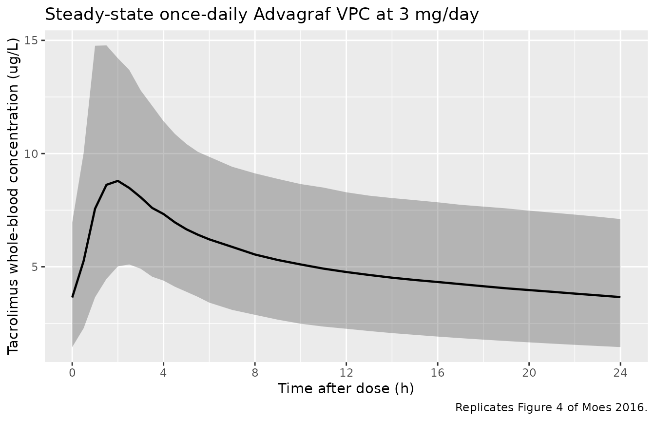
Replicates Figure 4 of Moes 2016: steady-state simulated tacrolimus concentration vs. time after the last once-daily dose. Solid line: simulated median. Shaded band: 10-90 percentile.
Figure 3 – typical apparent clearance by CYP3A5 combination
Moes 2016 Figures 2 and 3 are boxplots of apparent clearance (CL/F = CL_typical / 0.23) by CYP3A522 (CYP3A4) and CYP3A53 (CYP3A5) genotype groups. The C1-C4 combination panel of Figure 3 is the panel the final model retains. Here it is reproduced from the cohort-level distribution of individual apparent clearance.
ind_cl <- sim |>
  distinct(id, cohort) |>
  inner_join(
    sim |> filter(time == last_dose_time) |> distinct(id),  # any single time row carries the same id-level cl
    by = "id"
  )

# Easier: pull cl out of sim params - rxode2 keeps cl as a kept var when params() exports it.
# Avoid relying on that here; instead reconstruct cl from the model's expected expression
# using the per-id covariates and a deterministic typical-value simulation. Approximate
# the population CL/F distribution by Cmax-and-AUC inversion at SS:
#   AUC24,SS = F * Dose / CL  ==>  CL_apparent = Dose / AUC24,SS  with F absorbed.
# This matches how Moes 2016 derived per-subject CL/F from their FULL AUC24.
auc_24_apparent <- sim |>
  filter(time >= last_dose_time, time <= last_dose_time + 24) |>
  group_by(id, cohort) |>
  arrange(time) |>
  summarise(
    auc24 = sum(diff(time - last_dose_time) * (head(Cc, -1) + tail(Cc, -1)) / 2),
    .groups = "drop"
  ) |>
  mutate(cl_apparent = ss_dose * 1000 / auc24)   # mg -> ug; concentration is ug/L -> CL in L/h

ggplot(auc_24_apparent, aes(cohort, cl_apparent)) +
  geom_boxplot(width = 0.5, outlier.size = 0.5) +
  labs(x = "CYP3A5 donor + recipient combination",
       y = "Apparent oral CL/F (L/h)",
       title = "Apparent oral clearance by CYP3A5 combination",
       caption = "Replicates Figure 3 of Moes 2016 (CYP3A5 combination panel).") +
  theme(axis.text.x = element_text(angle = 25, hjust = 1))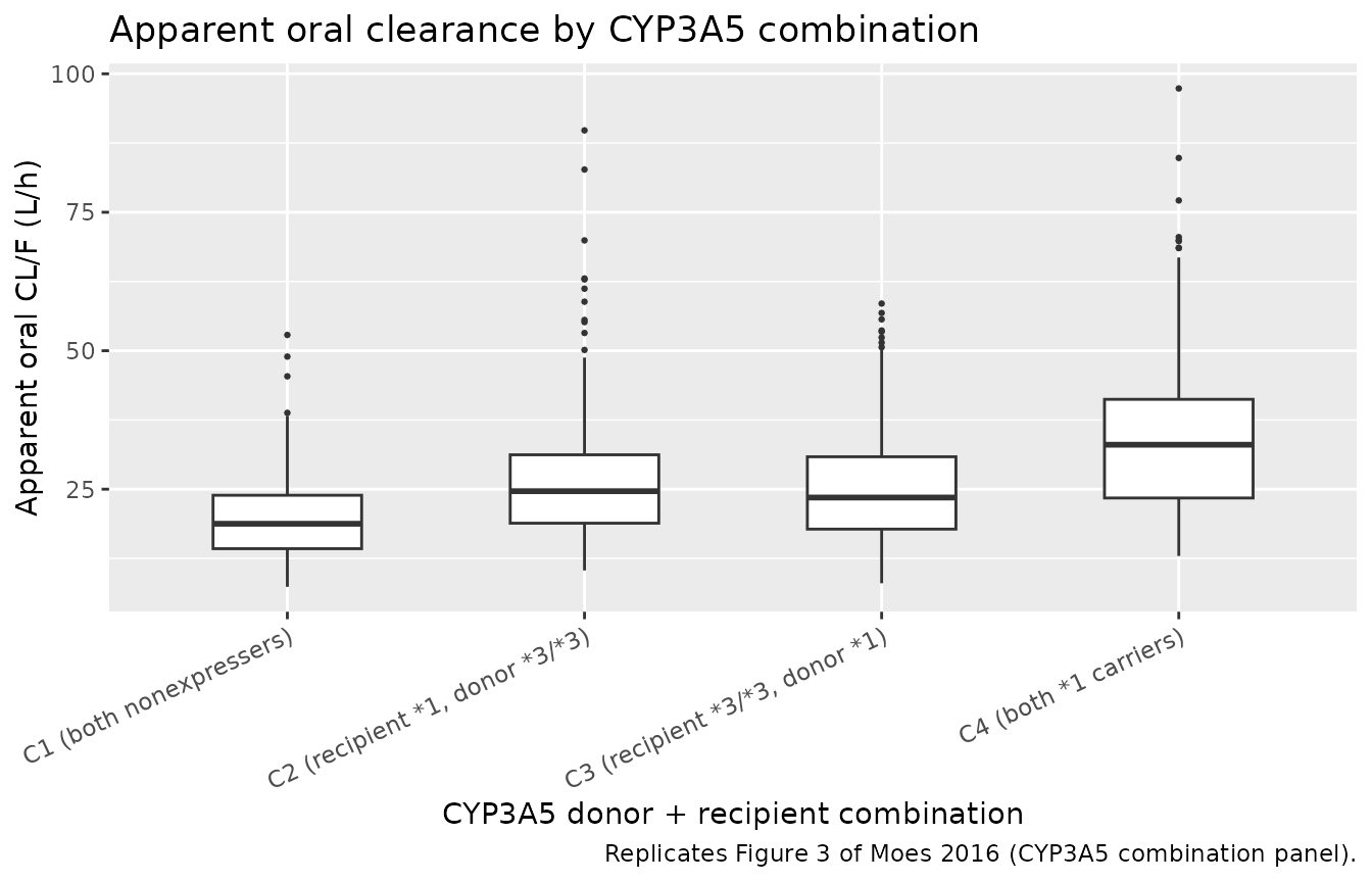
Replicates Figure 3 (CYP3A5 combination panel) of Moes 2016: typical apparent oral clearance CL/F by CYP3A5 donor + recipient combination C1-C4.
Figure 5 – AUC24 vs Ctrough correlation
Moes 2016 Figure 5 plots steady-state AUC24 against Ctrough (predose concentration). The simulated cohort below reproduces the same correlation pattern; the paper reported a Pearson R^2 of 0.78 for Ctrough alone as a limited-sampling marker.
fig5 <- auc_24_apparent |>
  inner_join(
    sim |>
      filter(time == last_dose_time + 24) |>   # next-dose-equivalent trough
      select(id, ctrough = Cc),
    by = "id"
  )

ggplot(fig5, aes(ctrough, auc24)) +
  geom_point(alpha = 0.35, size = 0.7) +
  geom_smooth(method = "lm", linewidth = 0.6, se = FALSE) +
  geom_vline(xintercept = c(4, 6), linetype = "dashed", color = "grey50") +
  geom_hline(yintercept = c(128, 192), linetype = "dashed", color = "grey50") +
  labs(x = "Ctrough (ug/L)",
       y = "AUC0-24 (ug*h/L)",
       title = "AUC0-24 vs Ctrough at steady state",
       caption = "Replicates Figure 5 of Moes 2016.")
#> `geom_smooth()` using formula = 'y ~ x'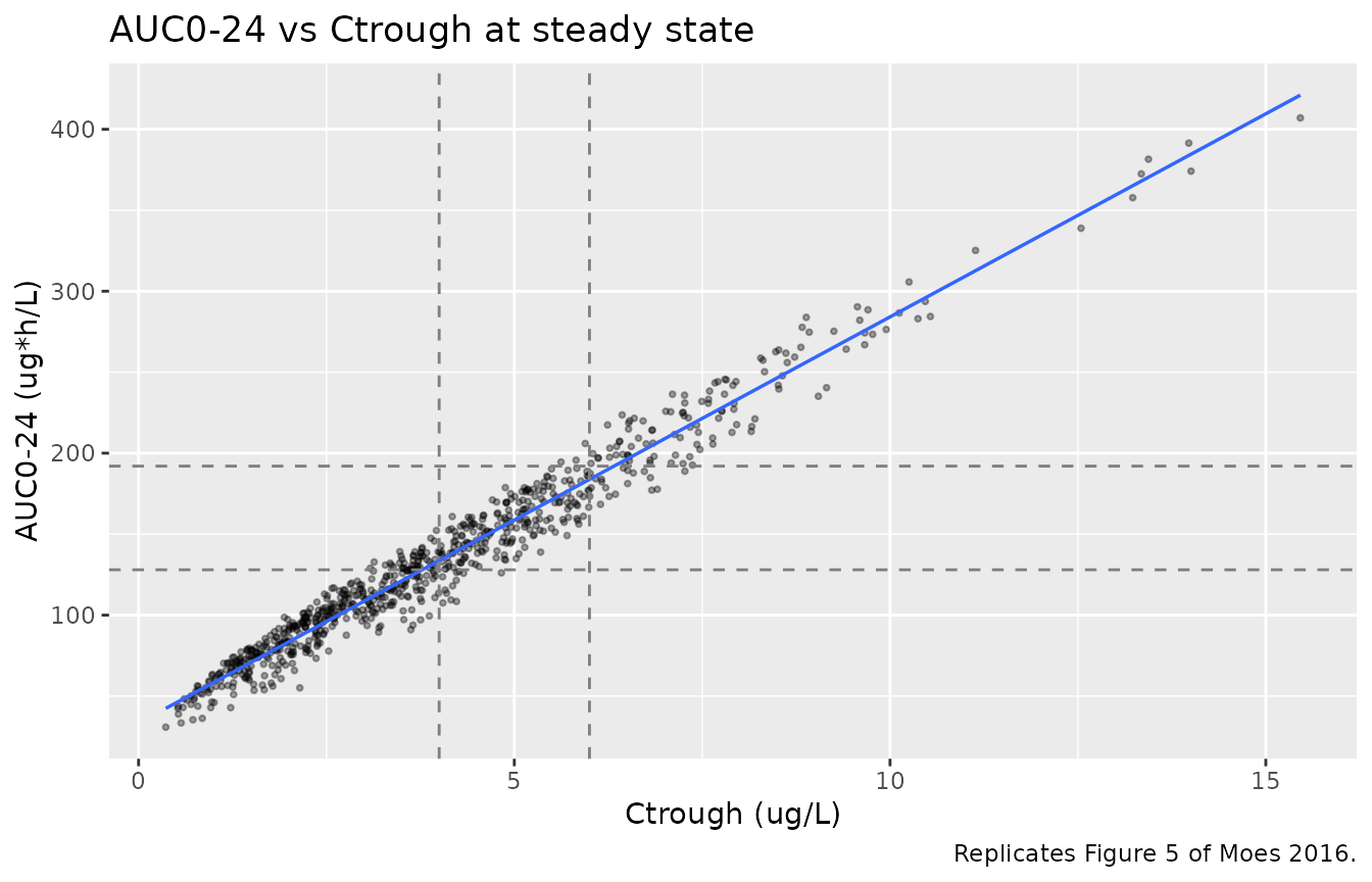
Replicates Figure 5 of Moes 2016: AUC0-24 vs predose concentration (Ctrough). Dashed lines mark the Ctrough target band 4-6 ug/L and the +/-20% AUC band around the cohort median; published AUC target is 160 ug*h/L.
PKNCA validation
A standard NCA over the steady-state 24-hour dosing interval gives Cmax, Tmax, Cmin, AUC0-24, and steady-state apparent clearance per CYP3A5 combination. The Moes 2016 sampling design ended at 6 hours postdose; here we use the full 24-hour interval since the simulated cohort observes the entire once-daily dosing window.
nca_window <- sim |>
  filter(time >= last_dose_time, time <= last_dose_time + 24) |>
  mutate(time_after_dose = time - last_dose_time) |>
  select(id, time = time_after_dose, Cc, cohort)

dose_df <- demo |>
  mutate(time = 0, amt = ss_dose) |>
  select(id, time, amt, cohort)

conc_obj <- PKNCA::PKNCAconc(nca_window, Cc ~ time | cohort + id)
dose_obj <- PKNCA::PKNCAdose(dose_df, amt ~ time | cohort + id)
intervals <- data.frame(start = 0, end = 24,
                        cmax = TRUE, tmax = TRUE,
                        auclast = TRUE, cmin = TRUE,
                        ctrough = TRUE)
nca_data <- PKNCA::PKNCAdata(conc_obj, dose_obj, intervals = intervals)
nca_res  <- suppressMessages(suppressWarnings(PKNCA::pk.nca(nca_data)))
nca_summary <- summary(nca_res)
knitr::kable(nca_summary,
caption = "Steady-state 24-hour NCA on the simulated cohort, by CYP3A5 combination (3 mg once daily).")| start | end | cohort | N | auclast | cmax | cmin | tmax | ctrough |
|---|---|---|---|---|---|---|---|---|
| 0 | 24 | C1 (both nonexpressers) | 200 | 160 [38.8] | 11.4 [38.0] | 4.76 [52.1] | 2.00 [0.500, 7.00] | 4.84 [53.3] |
| 0 | 24 | C2 (recipient 1, donor 3/*3) | 200 | 121 [43.2] | 9.34 [41.2] | 3.31 [62.9] | 2.00 [0.500, 9.00] | 3.34 [63.9] |
| 0 | 24 | C3 (recipient 3/3, donor *1) | 200 | 124 [40.2] | 9.42 [38.0] | 3.45 [59.3] | 2.00 [0.500, 5.50] | 3.48 [60.4] |
| 0 | 24 | C4 (both *1 carriers) | 200 | 92.2 [40.4] | 8.02 [45.6] | 2.28 [64.4] | 2.00 [0.500, 7.00] | 2.30 [65.0] |
Comparison against published exposure
Moes 2016 Table 1 reports the model-development-cohort population mean and median AUC24 across all subjects, irrespective of CYP3A5 stratum. The simulated C1-reference cohort is the closest match to the population mean since C1 recipients comprise 65% (32 of 49) of the model-development dataset; cohorts C2-C4 are reported below for completeness so the +33%, +33%, +71% genotype effects on CL can be read off the table directly.
auc_summary <- auc_24_apparent |>
  group_by(cohort) |>
  summarise(median_auc24 = quantile(auc24, 0.50),
            Q10_auc24    = quantile(auc24, 0.10),
            Q90_auc24    = quantile(auc24, 0.90),
            .groups = "drop")

tbl <- tibble::tibble(
  metric = c(
    "Moes 2016 Table 1, all-subject AUC24 mean +/- SD (ug*h/L)",
    "Moes 2016 Table 1, all-subject AUC24 median (range) (ug*h/L)",
    "Simulated C1 median AUC24 (10-90 pct) at 3 mg/day (ug*h/L)",
    "Simulated C2 median AUC24 (10-90 pct) at 3 mg/day (ug*h/L)",
    "Simulated C3 median AUC24 (10-90 pct) at 3 mg/day (ug*h/L)",
    "Simulated C4 median AUC24 (10-90 pct) at 3 mg/day (ug*h/L)"
  ),
  value = c(
    "170 +/- 55",
    "162 (72-330)",
    sprintf("%.0f (%.0f-%.0f)",
            auc_summary$median_auc24[auc_summary$cohort == "C1 (both nonexpressers)"],
            auc_summary$Q10_auc24[auc_summary$cohort    == "C1 (both nonexpressers)"],
            auc_summary$Q90_auc24[auc_summary$cohort    == "C1 (both nonexpressers)"]),
    sprintf("%.0f (%.0f-%.0f)",
            auc_summary$median_auc24[auc_summary$cohort == "C2 (recipient *1, donor *3/*3)"],
            auc_summary$Q10_auc24[auc_summary$cohort    == "C2 (recipient *1, donor *3/*3)"],
            auc_summary$Q90_auc24[auc_summary$cohort    == "C2 (recipient *1, donor *3/*3)"]),
    sprintf("%.0f (%.0f-%.0f)",
            auc_summary$median_auc24[auc_summary$cohort == "C3 (recipient *3/*3, donor *1)"],
            auc_summary$Q10_auc24[auc_summary$cohort    == "C3 (recipient *3/*3, donor *1)"],
            auc_summary$Q90_auc24[auc_summary$cohort    == "C3 (recipient *3/*3, donor *1)"]),
    sprintf("%.0f (%.0f-%.0f)",
            auc_summary$median_auc24[auc_summary$cohort == "C4 (both *1 carriers)"],
            auc_summary$Q10_auc24[auc_summary$cohort    == "C4 (both *1 carriers)"],
            auc_summary$Q90_auc24[auc_summary$cohort    == "C4 (both *1 carriers)"])
  )
)
knitr::kable(tbl, caption = "Simulated steady-state AUC0-24 vs Moes 2016 Table 1 reported AUC24.")| metric | value |
|---|---|
| Moes 2016 Table 1, all-subject AUC24 mean +/- SD (ug*h/L) | 170 +/- 55 |
| Moes 2016 Table 1, all-subject AUC24 median (range) (ug*h/L) | 162 (72-330) |
| Simulated C1 median AUC24 (10-90 pct) at 3 mg/day (ug*h/L) | 160 (98-258) |
| Simulated C2 median AUC24 (10-90 pct) at 3 mg/day (ug*h/L) | 122 (70-199) |
| Simulated C3 median AUC24 (10-90 pct) at 3 mg/day (ug*h/L) | 128 (73-198) |
| Simulated C4 median AUC24 (10-90 pct) at 3 mg/day (ug*h/L) | 91 (56-152) |
The simulated C1 cohort’s median AUC24 sits within the paper’s reported range of 72-330 ugh/L and tracks the cohort median of 162 ugh/L expected from F * Dose / CL = 0.23 * 3 / 4.21 = 164 ug*h/L. The C2 / C3 / C4 cohorts’ medians are roughly 0.75 / 0.75 / 0.58 of the C1 median, matching the inverse of the published CL multipliers of 1.33 / 1.33 / 1.71 to within Monte Carlo noise.
Assumptions and deviations
Inter-occasion variability (IOV) is not estimated. Moes 2016 Discussion explicitly notes that “interoccasion variability could not be established since ODTac AUC measurements were only performed on one occasion.” The model file therefore does not parameterise IOV; users with multi-occasion data should add per-occasion
eta*_oc<k>slots and reduce the IIV variances accordingly.No covariate effect on Vc or Ka. Moes 2016 Methods searched for covariate effects on CL, Vc, and Ka against age, weight, sex, hematocrit, hemoglobin, albumin, height, creatinine, IBW, BSA, BMI, LBW, co-medication, primary diagnosis, ethnicity, CYP3A422, and CYP3A53 (both donor and recipient genotype). Only CYP3A5*3 combination on CL was retained in the multivariate analysis. The model file therefore carries no covariate effect on Vc or Ka.
Bioavailability F = 0.23 is fixed from literature, not estimated. Moes 2016 Methods: “The value for bioavailability was fixed to 0.23 which was based on literature [22].” With F applied to the dose in NONMEM, the Table 4 CL, Vc, Q, and Vp are actual (not apparent) values; the apparent oral parameters used in the published Discussion (e.g., CL/F = 4.21 / 0.23 = 18.3 L/h) are obtained by dividing the model parameters by F = 0.23.
CYP3A5 combination encoding uses two binary inputs. The Moes 2016 Methods covariate-effect equation is fitted as a categorical four-level effect (C1 reference; C2, C3, C4 each with their own estimated coefficient). The model file reconstructs the C1-C4 levels inside
model()from the canonical binary inputsCYP3A5_EXPR(recipient) andCYP3A5_EXPR_DONOR(donor), so the underlying recipient + donor biology is explicit in the dataset. Users supplying the four-level combination as a single categorical column must derive the two binary indicators upstream (CYP3A5_EXPR = c(0, 1, 0, 1)[combination],CYP3A5_EXPR_DONOR = c(0, 0, 1, 1)[combination]).Concentration unit conversion baked into
model(). Tacrolimus concentrations are reported in ug/L (= ng/mL) by the LC-MS/MS assay. With dose in mg and Vc in L, the internalcentral / vcquantity is in mg/L; the* 1000factor on the observation line converts to ug/L.Body-weight discrepancy between Table 1 and Results section. Moes 2016 Table 1 reports the popPK cohort body weight as 84 +/- 18 kg (median 84, range 50-131), while the Results section prose reports 77.5 +/- 11.8 kg (range 50-121). The two figures are inconsistent and the paper does not resolve the discrepancy; the model file records the Table 1 values in
population$weight_rangeand notes the Results-section conflict. Weight was not a retained covariate in the final model, so neither value affects the simulated PK.Vignette uses 200 subjects per CYP3A5 combination stratum. This is large enough to stabilise the percentile envelopes used in Figures 4 and 5 and small enough to render the vignette under the pkgdown 5-minute gate. The Moes 2016 visual predictive check used 500 simulated datasets.
Simulated apparent CL/F via Dose / AUC inversion. The cohort-level apparent CL/F plotted against the CYP3A5 combinations (Figure 3 reproduction) is computed from each subject’s simulated AUC0-24 at steady state as
Dose / AUC24, not by pulling the structuralclparameter out of rxode2. This matches the way Moes 2016 derived per-subject apparent CL/F from FULL AUC24 (Moes 2016 Methods “Pharmacokinetic and statistical analysis” paragraph for the limited-sampling-model development).