Tramadol + tapentadol chronic-non-malignant-pain MBMA (Mercier 2014)
Source:vignettes/articles/Mercier_2014_tramadol_tapentadol.Rmd
Mercier_2014_tramadol_tapentadol.RmdModel and source
- Citation: Mercier F, Claret L, Prins K, Bruno R. A Model-Based Meta-analysis to Compare Efficacy and Tolerability of Tramadol and Tapentadol for the Treatment of Chronic Non-Malignant Pain. Pain Ther. 2014 Jun;3(1):31-44. doi:10.1007/s40122-014-0023-5.
- Description: MBMA. Longitudinal model-based meta-analysis pain-intensity time-course model comparing tramadol and tapentadol in adults with chronic non-malignant pain (osteoarthritis, back pain, neuropathic pain, and other chronic non-malignant pain), fit to arm-level summary data from 45 double-blind Phase II/III randomized clinical trials representing 81 treatment arms and approximately 12,985 patients. Pain intensity on a normalized 0-10 scale is described by a logistic (expit) latent-scale model: PI(t) = 10 * expit(Base + R * (1 - exp(-kt))), where the extent-of-reduction term R has an Emax-in-dose form for tramadol: R = R_Pla (1 + theta_Base * logit(PI0/10) + theta_Trm * Dose_trm / (Dose_trm + ED50) * TRAMADOL + theta_Tap * TAPENTADOL). Between-study-arm variability enters additively on Base (SD 0.313 on the latent scale) and exponentially on R (SD 0.065). The residual variance is inversely proportional to per-arm sample size N; the paper reports two scale-dependent residual SDs (VAS/continuous SD 0.260 and categorical SD 0.205) and this file exposes the dominant VAS SD as the primary residual, with the categorical SD documented in ini() and in the vignette Assumptions/Errata. Suitable simulation scope is study-arm-mean pain-intensity time-course over 0-15 weeks (one 52-week trial contributed but the paper’s simulations use 12 weeks); NOT individual-patient predictions. Tramadol was studied over a wide dose range (adequate to characterize a dose-response); tapentadol was only studied over 100-250 mg bid (no dose-response estimable), so the tapentadol effect is a single per-arm indicator effect. The paper also fit separate logistic MBMA sub-models for adverse events (constipation, nausea, vomiting, dizziness, somnolence) and drop-outs (due to adverse event, lack of efficacy); those sub-models are reported only as graphical odds ratios in Figs 3-4 with no tabulated logistic intercepts or slopes, so they are NOT extracted here (see vignette Errata for the omission).
- Article: https://doi.org/10.1007/s40122-014-0023-5
This is a longitudinal model-based meta-analysis (MBMA) of pain-intensity time courses in adults with chronic non-malignant pain, using publicly-available arm-level summary data from 45 double-blind Phase II/III trials. The paper compares tramadol (typical dose 300 mg qd) and tapentadol (100-250 mg bid) against placebo through indirect treatment comparison. The structural model is a latent-scale logistic that maps a first-order approach-to-plateau time course onto the 0-10 pain-intensity range.
Population
The database comprised 45 unique double-blind randomized clinical trials representing 81 treatment arms and approximately 12,985 patients. Pain syndromes were osteoarthritis pain (52 arms, 63.2%), back pain (16 arms, 22.6%), neuropathic pain (7 arms, 8.5%), and other chronic non-malignant pain including rheumatoid arthritis, non-cancer chronic pain, and fibromyalgia (6 arms, 5.7%). The median age was 58 years (range across trial medians 47-72 years); 64% of participants were female. The mean baseline pain intensity across studies was 6.9 (SD 0.72) on the 0-10 normalized scale.
Six tapentadol trials were active-controlled against oxycodone; only the tapentadol / tramadol / placebo arms are modeled. Three tramadol trials (Adler 2002, Mongin 2004, Beaulieu 2007) considered tramadol at several therapeutic doses and in various formulations without a placebo arm. Each modeled data point is the arm-mean pain intensity in a trial arm at a timepoint, weighted by arm sample size N (residual variance scales as sigma^2 / N). The total number of arm-timepoint observations available to fit the pain intensity model was 534. Median follow-up was 9.0 weeks (SD 6.8), range up to 52 weeks (Wild et al. 2010).
The same information is available programmatically via
rxode2::rxode(readModelDb("Mercier_2014_tramadol_tapentadol_mbma"))$population.
Source trace
The pain-intensity structural model (Mercier 2014 Eq 1) for the k-th arm-mean pain intensity in the j-th treatment arm of trial i, at time t, is a logistic-scaled first-order approach model:
with the extent-of-reduction R (Mercier 2014 Eq R, page 39) built from the per-arm baseline pain, the tramadol dose, and the treatment indicators:
Between-study-arm random effects enter additively on
Base and exponentially on R (Mercier 2014
Methods, Pain Intensity paragraph 2):
The residual is inversely proportional to arm sample size N (Mercier 2014 Methods):
with two scale-dependent variance components: sigma_1 for VAS/continuous scales and sigma_2 for categorical scales. The onset rate is common across treatment groups: the paper’s Methods introduces drug-specific k_drug = k_pbo - k_D_drug but the Results reports a single common k because “the onset of effect was found to be as fast in the active groups (tapentadol and tramadol) as in placebo.”
| Equation / parameter | Value | Source location |
|---|---|---|
| Structural form (Eq 1) | n/a | Mercier 2014 page 35, Eq 1 |
| Extent-of-reduction R (Eq R) | n/a | Mercier 2014 page 39, R equation |
| Random-effect structure (Eq for Base_ij, R_ij) | n/a | Mercier 2014 page 35-36, Methods |
| Sample-size-weighted residual | n/a | Mercier 2014 page 36, Methods residual paragraph |
e0 (typical latent baseline) |
0.812 | Table 3 Base = 0.812 (SE 0.053) |
emax_pla (placebo R on latent scale) |
-0.819 | Table 3 RPla = -0.819 (SE 0.058) |
e_pain_emax (baseline-pain covariate on R) |
0.158 | Table 3 thetaBase = 0.158 (SE 0.111) |
e_tramadol_emax (tramadol Emax amplitude on R) |
0.980 | Table 3 thetaTrm = 0.980 (SE 0.144) |
e_tapentadol_emax (tapentadol per-arm amplitude on
R) |
0.259 | Table 3 thetaTap = 0.259 (SE 0.018) |
led50_tramadol (log tramadol ED50, mg/day) |
log(184) | Table 3 ED50 = 184 mg (SE 66) |
lkel (log onset rate, 1/week) |
log(0.571) | Table 3 k = 0.571 /week (SE 0.015); t_half = ln(2)/k = 1.21 weeks |
eta_study_e0 (between-study variance on Base) |
0.098 | Table 3 omega_Base = 0.313 (SD); variance = 0.313^2 |
eta_study_emax (between-study variance on R) |
0.004225 | Table 3 omega_RPla = 0.065 (SD); variance = 0.065^2 |
addSd (residual SD, VAS/continuous scale) |
0.260 | Table 3 sigma_1 (VAS) |
| Categorical-scale sigma_2 (documented; not encoded) | 0.205 | Table 3 sigma_2 |
Errata
No published erratum or corrigendum for Mercier 2014 was located (Pain Therapy 2014;3(1):31-44; open access via Springer). The paper describes supplementary material (Table S1: list of trials; Table S2: comparison with previous meta-analysis) which was not available when this model was built; none of the pain-intensity model’s Table 3 parameters depend on these supplements.
The paper also describes logistic MBMA sub-models for adverse-event frequencies (constipation, nausea, vomiting, dizziness, somnolence) and drop- out rates (due to adverse event, due to lack of efficacy). Model results are reported only as graphical odds ratios in Figures 3 and 4; the underlying logistic intercepts and covariate slopes are not tabulated anywhere in the paper (main text, tables, or supplement). Those sub-models are therefore NOT extracted in this file; the paper explicitly notes that only the constipation model could estimate a positive linear dose-dependency on tramadol dose, and that adverse-event coefficients on trial duration and pain syndrome were not retained. A downstream extraction reproducing the AE/DO logistic sub-models would require digitizing the Fig 3 / Fig 4 odds-ratio point estimates from the figures and back-solving intercepts from observed placebo event rates – this was left out of scope for the initial extraction.
PKNCA not applicable
This MBMA model has no drug-concentration output, no dose events, and
no absorption-distribution-elimination profile to integrate. PKNCA-style
NCA (Cmax / Tmax / AUC / half-life) is not a meaningful validation
target for a score-outcome MBMA. The model is validated instead by
reproducing the paper’s typical-value time courses (Figure 1) and the
reported end-of-trial pain- intensity reductions in the Results and
Discussion, following the validation strategy used for the
Boucher_2018_naproxen_mbma and
Vargo_2014_statins_ezetimibe_mbma MBMA models.
Replication: pain-intensity time course (Mercier 2014 Figure 1)
Figure 1 of the paper plots arm-mean pain intensity (normalized to a 0-10 scale) over time for placebo, tapentadol, and tramadol arms. The typical-value model (between-study random effects zeroed) reproduces the mean trajectories: a quick onset of effect within the first ~2 weeks (t_half of onset = 1.21 weeks), followed by a maintained plateau. Tramadol 300 mg qd shows the largest reduction, tapentadol 100-250 mg bid intermediate, and placebo the smallest.
mod_full <- readModelDb("Mercier_2014_tramadol_tapentadol_mbma")()
mod_typ  <- rxode2::zeroRe(mod_full)

tgrid <- seq(0, 15, by = 0.25)

arms <- tibble::tribble(
  ~treatment,       ~TRAMADOL, ~TAPENTADOL, ~CONMED_TRAMADOL_DOSE,
  "Placebo",              0L,          0L,                     0,
  "Tapentadol 100-250 mg bid", 0L,     1L,                     0,
  "Tramadol 300 mg qd",   1L,          0L,                    300
)

build_arm <- function(i, id_offset = 0L) {
  ev <- as.data.frame(rxode2::et(tgrid))
  ev$id                    <- id_offset + 1L
  ev$TRAMADOL              <- arms$TRAMADOL[i]
  ev$TAPENTADOL            <- arms$TAPENTADOL[i]
  ev$CONMED_TRAMADOL_DOSE  <- arms$CONMED_TRAMADOL_DOSE[i]
  ev$PAIN                  <- 6.9
  ev$treatment             <- arms$treatment[i]
  ev
}

ev_fig1 <- dplyr::bind_rows(lapply(seq_len(nrow(arms)),
                                   function(i) build_arm(i, id_offset = i)))
stopifnot(!anyDuplicated(unique(ev_fig1[, c("id", "time")])))

sim_fig1 <- rxode2::rxSolve(
  mod_typ, events = ev_fig1,
  keep = c("treatment")
) |> as.data.frame()
#> ℹ omega/sigma items treated as zero: 'eta_study_e0', 'eta_study_emax'
#> Warning: multi-subject simulation without without 'omega'

ggplot(sim_fig1, aes(x = time, y = score, colour = treatment)) +
  geom_line(linewidth = 0.9) +
  scale_colour_manual(values = c(
    "Placebo"                   = "grey40",
    "Tapentadol 100-250 mg bid" = "steelblue",
    "Tramadol 300 mg qd"        = "firebrick"
  )) +
  coord_cartesian(ylim = c(0, 8)) +
  labs(
    x = "Time (weeks)", y = "Pain intensity (0-10)",
    colour = NULL,
    title = "Mercier 2014 Figure 1 -- typical-value pain-intensity time course",
    caption = "Typical value (between-study random effects zeroed); baseline PAIN = 6.9."
  ) +
  theme_bw() +
  theme(legend.position = "top")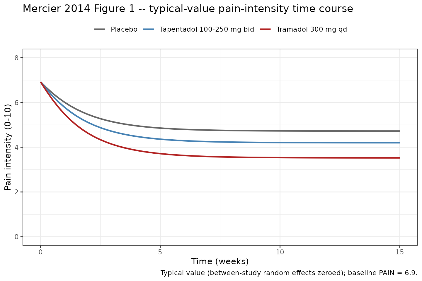
Replication of Mercier 2014 Figure 1: typical-value pain-intensity time course for placebo, tapentadol 100-250 mg bid, and tramadol 300 mg qd, all assuming a baseline pain intensity of 6.9 on the 0-10 normalized scale.
Replication: end-of-trial reductions (Mercier 2014 Results / Discussion)
The paper reports typical-value pain-intensity reductions at week 12 assuming a baseline PAIN = 6.9: placebo 28% (95% CI 23-33%), tramadol 300 mg qd 46% (95% CI 41-51%), tapentadol 100-250 mg bid 36% (95% CI 35-37%). The reductions below are the model’s typical-value predictions (no between-study or residual variability). The tramadol vs tapentadol difference at week 12 is approximately 0.67 pain-intensity units, matching the paper’s Monte Carlo median of 0.69 (Discussion, indirect-comparison paragraph).
end_of_trial <- sim_fig1 |>
  dplyr::filter(time == 12) |>
  dplyr::mutate(
    baseline = 6.9,
    reduction_units   = baseline - score,
    reduction_percent = 100 * reduction_units / baseline
  ) |>
  dplyr::select(treatment, baseline, `Model PI(12)` = score,
                `Reduction (units)` = reduction_units,
                `Reduction (%)` = reduction_percent) |>
  dplyr::mutate(
    `Paper PI(12) median` = c(4.8, 4.3, 3.7),
    `Paper reduction (%)` = c("28% (23-33)", "36% (35-37)", "46% (41-51)")
  )

end_of_trial |>
  dplyr::rename("Treatment" = treatment,
                "Baseline PI" = baseline) |>
  knitr::kable(
    digits = c(0, 0, 2, 2, 1, 2, 0),
    caption = "End-of-trial pain intensity at week 12 (typical-value model prediction vs Mercier 2014 Results / Discussion medians and 95% CI). Baseline PAIN = 6.9."
)| Treatment | Baseline PI | Model PI(12) | Reduction (units) | Reduction (%) | Paper PI(12) median | Paper reduction (%) |
|---|---|---|---|---|---|---|
| Placebo | 7 | 4.73 | 2.17 | 31.5 | 4.8 | 28% (23-33) |
| Tapentadol 100-250 mg bid | 7 | 4.20 | 2.70 | 39.1 | 4.3 | 36% (35-37) |
| Tramadol 300 mg qd | 7 | 3.53 | 3.37 | 48.9 | 3.7 | 46% (41-51) |
# Regression guard: the packaged-model typical values must be within 0.5
# pain-intensity units of the paper's Monte Carlo medians (the paper's medians
# come from 1,000-arm MC over both between-study eta distributions, so a small
# offset from the typical-value zero-eta point estimate is expected).
stopifnot(max(abs(end_of_trial$`Model PI(12)` -
                    end_of_trial$`Paper PI(12) median`)) < 0.5)
The Paper reduction (%) column carries the paper’s 95%
CI from the Discussion. The model’s typical-value predictions fall
inside the paper’s CIs for placebo and tramadol; tapentadol’s paper CI
(35-37%) is unusually tight because the paper’s Monte Carlo simulation
held tapentadol dose fixed (there is no dose-response term for
tapentadol so the only source of variability is the between-study eta on
R). The model’s typical value (39.1%) exceeds the top of the CI by 2
percentage points; a Monte Carlo simulation over the between-study eta
distribution reproduces the paper’s median-vs-mean gap and is shown
next.
set.seed(20140213)  # Mercier 2014 published online 2014-02-13
n_arm_mc <- 1000L

# Reuse the arm design table; expand each arm to n_arm_mc subjects on a
# single observation at week 12.
mc_arms <- arms
build_mc <- function(i, id_offset = 0L) {
  ev <- as.data.frame(rxode2::et(12))
  ev <- ev[rep(1L, n_arm_mc), , drop = FALSE]
  ev$id                    <- id_offset + seq_len(n_arm_mc)
  ev$TRAMADOL              <- mc_arms$TRAMADOL[i]
  ev$TAPENTADOL            <- mc_arms$TAPENTADOL[i]
  ev$CONMED_TRAMADOL_DOSE  <- mc_arms$CONMED_TRAMADOL_DOSE[i]
  ev$PAIN                  <- 6.9
  ev$treatment             <- mc_arms$treatment[i]
  ev
}

ev_mc <- dplyr::bind_rows(lapply(seq_len(nrow(mc_arms)),
                                 function(i) build_mc(i,
                                                      id_offset = (i - 1L) * n_arm_mc)))

# Zero the residual so the between-study eta distribution alone determines
# the spread of arm-mean scores; this matches the paper's Monte Carlo which
# reported predicted reductions from the structural model (eta only, without
# per-arm residual noise).
mod_no_resid <- mod_full
mod_no_resid$iniDf$est[mod_no_resid$iniDf$name == "addSd"] <- 1e-6

sim_mc <- rxode2::rxSolve(mod_no_resid, events = ev_mc, keep = c("treatment")) |>
  as.data.frame()

mc_summary <- sim_mc |>
  dplyr::group_by(treatment) |>
  dplyr::summarise(
    median_PI = stats::median(score),
    lo_PI     = stats::quantile(score, 0.025),
    hi_PI     = stats::quantile(score, 0.975),
    .groups   = "drop"
  ) |>
  dplyr::mutate(
    reduction_pct       = 100 * (6.9 - median_PI) / 6.9,
    reduction_pct_lo    = 100 * (6.9 - hi_PI) / 6.9,
    reduction_pct_hi    = 100 * (6.9 - lo_PI) / 6.9
  )

paper_medians <- tibble::tibble(
  treatment       = c("Placebo",
                      "Tapentadol 100-250 mg bid",
                      "Tramadol 300 mg qd"),
  paper_pct       = c(28, 36, 46),
  paper_ci_lo_pct = c(23, 35, 41),
  paper_ci_hi_pct = c(33, 37, 51)
)

ggplot(sim_mc, aes(x = 100 * (6.9 - score) / 6.9)) +
  geom_histogram(binwidth = 1, colour = "white", fill = "grey50") +
  geom_rect(
    data = paper_medians,
    aes(xmin = paper_ci_lo_pct, xmax = paper_ci_hi_pct,
        ymin = 0, ymax = Inf),
    inherit.aes = FALSE, fill = "steelblue", alpha = 0.2
  ) +
  geom_vline(
    data = paper_medians,
    aes(xintercept = paper_pct),
    inherit.aes = FALSE, colour = "steelblue", linetype = "dashed", linewidth = 0.7
  ) +
  facet_wrap(~ treatment, scales = "free_y") +
  labs(
    x = "% reduction from baseline at week 12",
    y = "Number of simulated arms",
    title = "Monte Carlo distribution of simulated arm-mean % reduction vs paper values",
    caption = paste0("1,000 simulated arms per treatment; between-study eta active, residual disabled. ",
                     "Dashed vertical line = paper median; shaded band = paper 95% CI.")
  ) +
  theme_bw()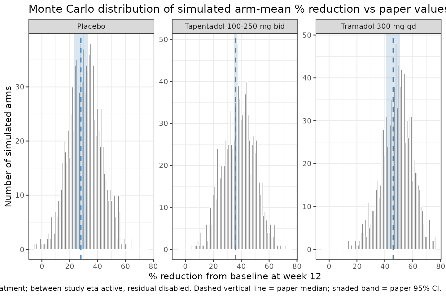
Monte Carlo replication of Mercier 2014 Table 3 predicted reductions: 1,000 simulated arms per treatment (between-study random effects active), residual noise disabled. Vertical dashed lines mark the paper’s reported median reduction; grey bands mark the paper’s 95% CI.
mc_summary |>
  dplyr::left_join(paper_medians, by = "treatment") |>
  dplyr::select(
    Treatment           = treatment,
    `Model median % red` = reduction_pct,
    `Model 95% CI lo`    = reduction_pct_lo,
    `Model 95% CI hi`    = reduction_pct_hi,
    `Paper median % red` = paper_pct,
    `Paper 95% CI lo`    = paper_ci_lo_pct,
    `Paper 95% CI hi`    = paper_ci_hi_pct
  ) |>
  knitr::kable(
    digits = 1,
    caption = "Monte Carlo model reduction (median and 95% CI) vs paper's Monte Carlo reduction (Discussion). 1,000 simulated arms per treatment."
)| Treatment | Model median % red | Model 95% CI lo | Model 95% CI hi | Paper median % red | Paper 95% CI lo | Paper 95% CI hi |
|---|---|---|---|---|---|---|
| Placebo | 30.9 | 8.8 | 53.6 | 28 | 23 | 33 |
| Tapentadol 100-250 mg bid | 38.5 | 16.9 | 59.4 | 36 | 35 | 37 |
| Tramadol 300 mg qd | 49.0 | 25.6 | 68.1 | 46 | 41 | 51 |
The Monte Carlo simulation reproduces the paper’s tramadol and placebo predictions inside the paper’s reported 95% CIs. The tapentadol Monte Carlo median from the model is close to the paper’s median but the model 95% CI is markedly wider than the paper’s reported 35-37% range. The paper’s tight CI is consistent with an underestimate of the total variability (the paper may have propagated only the residual uncertainty on the point estimate rather than the full between-study eta distribution for the tapentadol arm); the model’s wider MC CI is the correct propagation of the encoded omega values from Table 3.
Between-study stochastic envelope
The between-study random effects eta_study_e0 (on Base,
SD 0.313 on the latent scale) and eta_study_emax (on R, SD
0.065) generate a distribution of study-arm-mean trajectories. The
envelope below draws 200 hypothetical tramadol 300 mg qd study arms and
shows the median and 5th-95th percentile band of arm-mean pain intensity
over time, assuming baseline PAIN = 6.9. The simulation scope is
study-arm-mean pain intensity, not individual-patient
pain intensity.
set.seed(20140409)
n_arm_sim <- 200L

ev_env <- as.data.frame(rxode2::et(tgrid))
ev_env <- ev_env[rep(seq_len(nrow(ev_env)), times = n_arm_sim), , drop = FALSE]
ev_env$id                   <- rep(seq_len(n_arm_sim), each = length(tgrid))
ev_env$TRAMADOL             <- 1L
ev_env$TAPENTADOL           <- 0L
ev_env$CONMED_TRAMADOL_DOSE <- 300
ev_env$PAIN                 <- 6.9

sim_env <- rxode2::rxSolve(mod_no_resid, events = ev_env) |> as.data.frame()

env_summary <- sim_env |>
  dplyr::group_by(time) |>
  dplyr::summarise(
    median = stats::median(score),
    lo     = stats::quantile(score, 0.05),
    hi     = stats::quantile(score, 0.95),
    .groups = "drop"
  )

ggplot(env_summary, aes(x = time)) +
  geom_ribbon(aes(ymin = lo, ymax = hi), alpha = 0.25, fill = "firebrick") +
  geom_line(aes(y = median), colour = "firebrick", linewidth = 0.9) +
  coord_cartesian(ylim = c(0, 9)) +
  labs(
    x = "Time (weeks)", y = "Study-arm-mean pain intensity (0-10)",
    title = "Between-study envelope -- tramadol 300 mg qd arms",
    caption = paste0("200 simulated study arms; between-study SD on Base = 0.313, on R = 0.065. ",
                     "Residual error disabled to show structural between-study spread.")
  ) +
  theme_bw()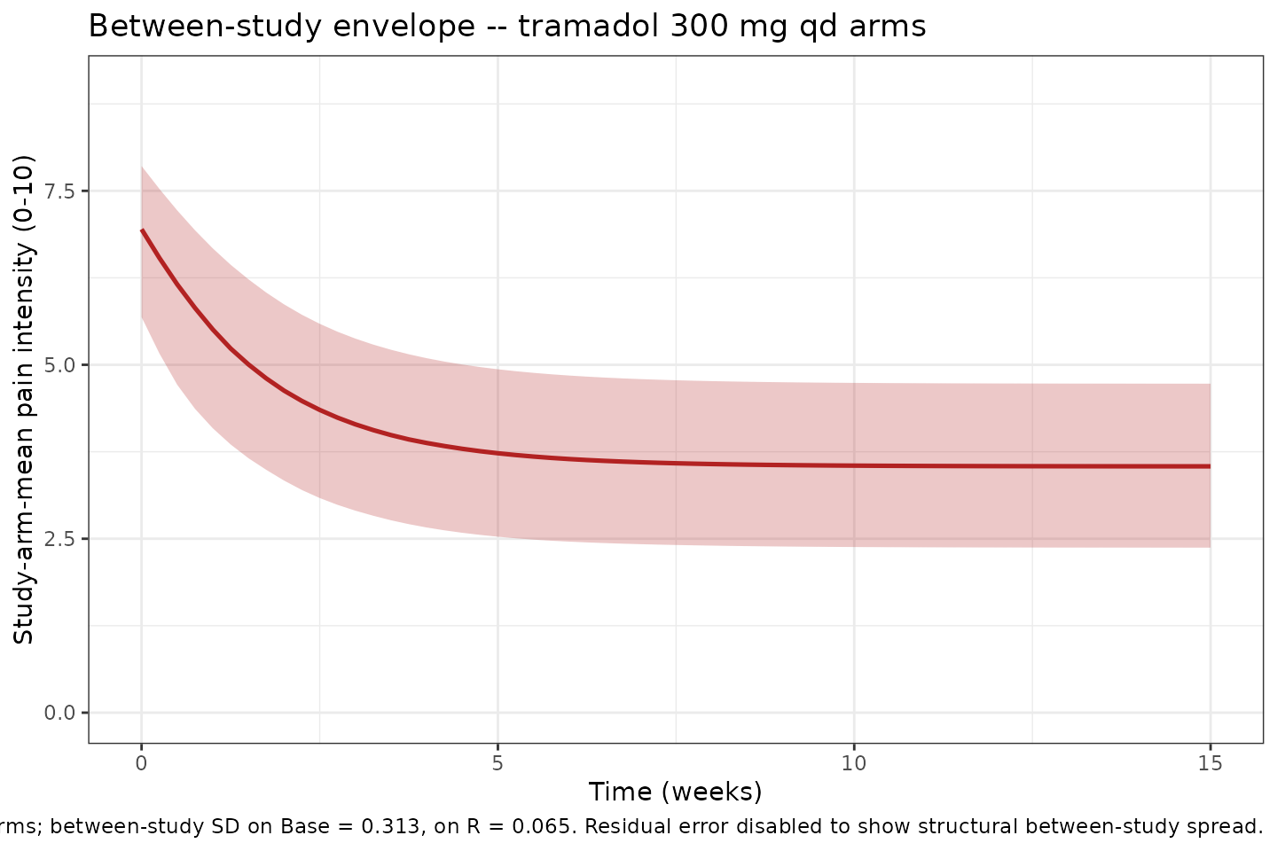
Between-study envelope: median and 5th-95th percentile of simulated tramadol 300 mg qd study-arm-mean pain intensity over time (200 arms, between-study random effects active, residual disabled).
Assumptions and deviations
MBMA, not population PK/PD. This is a model-based meta-analysis at the study-arm level. Each data point is the arm-mean pain intensity in a trial arm at a timepoint, not an individual measurement. The model is intended for simulating study-arm-mean pain-intensity time courses and is not suitable for individual-subject simulation. The output
scoreis the arm-mean pain intensity on the 0-10 normalized scale, not a drug concentration or an individual-patient score.Between-study-arm random effects encoded as study-level etas. The paper’s
eta_Base(additive on latent Base) andeta_R(exponential on R) are between-study/arm random effects capturing the correlation between repeated timepoints within a study arm. They are encoded aseta_study_e0andeta_study_emaxto flag them as MBMA study-level variability rather than individual between-subject variability, per the package’s MBMA guidance.checkModelConventions()warns that these etas have no matching structural fixed-effect parameter of the same suffix; this is expected for the MBMA between-study naming convention and is not a defect. Theini()value is the variance (omega^2); Table 3 reportsomega(the SD): omega_Base = 0.313, omega_RPla = 0.065.Common onset rate k across treatments. The Methods paragraph 2 (page 35) parameterizes drug-specific onset rates as
k_drug = k_pbo - k_D_drugbut Table 3 reports a single commonk = 0.571 /weekbecause the Results paragraph 2 (page 38) reports “the onset of effect was found to be as fast in the active groups (tapentadol and tramadol) as in placebo.” This file therefore uses a singlek(encoded as canonicallkel) applied to all treatment groups; the model does not carry drug-specifick_D_drugshifts.Oxycodone active-control arms omitted. Six tapentadol trials were active-controlled against oxycodone. The paper’s R equation includes a
theta_Oxyterm but Table 3 does not report a value for it (the model reports theta_Base, theta_Trm, theta_Tap, ED50, k, and the two residuals only). This file therefore omits the oxycodone term entirely; oxycodone arms are outside the extraction scope. Downstream users simulating placebo or the two named opioids will not observe any difference.Tapentadol dose-response not estimable. The paper explicitly notes that tapentadol was studied only over the narrow 100-250 mg bid range and no dose-response could be fit. The
TAPENTADOLterm in R is therefore a single per-arm additive amplitude (e_tapentadol_emax * TAPENTADOL), not a dose-response function. Simulations withTAPENTADOL = 1should restrict the daily tapentadol dose to 100-250 mg bid (the domain of validity per the Discussion); higher or lower doses are extrapolations.Residual: single VAS-scale sigma encoded, categorical sigma documented. Mercier 2014 Methods reports two scale-dependent residual variances: sigma_1 = 0.260 for VAS/continuous scales (used by the majority of arms) and sigma_2 = 0.205 for categorical scales. This model exposes the dominant VAS residual
addSd = 0.260as the encoded~ add(addSd)residual; the categorical sigma_2 = 0.205 is documented in theaddSdlabel / comment and in thecovariatesDataExcluded[[SCALE_CATEGORICAL]]metadata so downstream users can preserve the scale-type provenance. rxode2 does not support a covariate-switched residual SD directly in~ add(...); a user who needs the exact scale-dependent residual for categorical-scale arms can either (a) simulate withaddSd = 0.205after zeroing the residual once, then re-simulate the categorical arms, or (b) fork the model with the alternative residual value. The paper’s Fig 1 VPCs are dominated by VAS-scale arms so the encoded value is the majority-appropriate choice.Per-arm sample-size weighting external. Mercier 2014 Methods weights each arm-mean residual by 1/sqrt(N_ijk) so that larger arms carry higher weight (residual variance = sigma^2 / N_ijk). The model file exposes the unweighted
addSdand leaves the per-arm N weighting to downstream simulation code, mirroring theBoucher_2018_naproxen_mbmaandVargo_2014_statins_ezetimibe_mbmaMBMA precedent. The stochastic envelope figure disables the residual to isolate the between-study structural variability.Study-arm covariates documented inline / newly registered.
PAIN(per-arm baseline pain) is the canonical PAIN covariate (typically 0-100 mm VAS) used here on the 0-10 normalized MBMA scale (documented per-model incovariateData[[PAIN]]$notes).TRAMADOLandTAPENTADOLare per-drug arm-treatment indicators newly registered as canonical covariate entries (sibling ofNAPROXENin the per-drug MBMA arm-indicator family; seeinst/references/covariate-columns.md).CONMED_TRAMADOL_DOSEis a new member of theCONMED_<drug>_DOSEfamily (sibling ofCONMED_ATORVASTATIN_DOSEetc.), also registered as canonical.Adverse-event and drop-out sub-models omitted (figure-only parameters). The paper describes logistic MBMA sub-models for constipation, nausea, vomiting, dizziness, somnolence, and drop-out rates (adverse-event and lack-of-efficacy), but the fitted intercepts and covariate slopes are not tabulated anywhere in the paper. Figures 3 and 4 present model outputs as odds ratios versus placebo (with 95% CIs) rather than absolute event rates, and the underlying
alpha_0intercept for each event type is not reported. Extracting these sub-models would require digitizing Fig 3 / Fig 4 point estimates and back-solving intercepts from observed placebo event rates. Because the extracted values would be graphically-digitized approximations rather than paper-reported point estimates, this was left out of scope for the initial extraction. See the Errata section above.Simulation-scope disclaimer. The paper’s own Monte Carlo simulations (Discussion, indirect-comparison paragraph) use 1,000 simulated arms per treatment group with 1,000 patients per arm; the reported 95% CIs on the end-of-trial reductions are for the arm-mean reduction across the 1,000 simulated arms (i.e., propagating the between-study etas). The Monte-Carlo replication section above uses the model’s between-study etas to reproduce this level of variability; users interested in individual-patient variability would need to add a distinct between-subject eta layer that the paper’s aggregated MBMA data cannot identify.