Spatholobi Caulis active constituents (Liu 2024)
Source:vignettes/articles/Liu_2024_spatholobiCaulis.Rmd
Liu_2024_spatholobiCaulis.RmdModel and source
- Article: Pharmaceuticals 2024;17(12):1621
- Supplement:
pharmaceuticals-17-01621-s001.zip(open access, published with the article,PMC11677527)
Liu 2024 studies four active constituents of Spatholobi Caulis (SPC), a traditional Chinese medicine derived from the dried tuber of Spatholobus suberectus Dunn. Rats received a single oral gavage of SPC aqueous extract; the plasma concentrations of 3’-methoxydaidzein, 8-O-methylretusin, daidzin and isolariciresinol were measured by UFLC-MS/MS.
The paper’s headline model is a whole-body physiologically based pharmacokinetic (PBPK) model built in GastroPlus 9.8.2. That layer is not packaged here – see What is not extracted below. What is packaged is the compartmental model that the authors fitted to their own validation experiment with Drug and Statistics (DAS) v2.0 and tabulated in Supplementary Tables S3, S5, S7 and S9: a two-compartment oral model with first-order absorption and no lag time, one per constituent.
modelNames <- c(
  "3'-methoxydaidzein" = "Liu_2024_3methoxydaidzein_rat",
  "8-O-methylretusin"  = "Liu_2024_8Omethylretusin_rat",
  "daidzin"            = "Liu_2024_daidzin_rat",
  "isolariciresinol"   = "Liu_2024_isolariciresinol_rat"
)
uis <- lapply(modelNames, function(nm) rxode2::rxode(readModelDb(nm)))

tibble(
  Constituent = names(modelNames),
  `Model file` = unname(modelNames)
) |>
knitr::kable()| Constituent | Model file |
|---|---|
| 3’-methoxydaidzein | Liu_2024_3methoxydaidzein_rat |
| 8-O-methylretusin | Liu_2024_8Omethylretusin_rat |
| daidzin | Liu_2024_daidzin_rat |
| isolariciresinol | Liu_2024_isolariciresinol_rat |
Citation (identical for all four models):
cat(uis[[1]]$reference)Liu X, Du R, Zhang T, Li Y, Li L, Yang Z, Zhang Y, Wang Q (2024). Predicting pharmacokinetics of active constituents in Spatholobi caulis by using physiologically based pharmacokinetic models. Pharmaceuticals (Basel) 17(12):1621. doi:10.3390/ph17121621
Population
Liu 2024 Section 4.2.5 describes the validation experiment reproduced in this vignette: rats were given 1.5 mL of SPC suspension by gavage at 60 g crude drug/kg body weight, and 300 uL of orbital venous blood was sampled at 0.083, 0.25, 0.5, 0.75, 1.0, 1.5, 2, 3, 4, 6, 8 and 12 h. Supplementary Table S2 states “Parallel rats: 5”, so each concentration is the mean of five animals. The constituent doses delivered by that SPC dose are 0.124, 0.22, 1.4 and 2.62 mg/kg respectively.
The paper does not restate the rat strain, sex, age or body weight; those are recorded in the authors’ earlier study (Liu 2021, J Pharm Biomed Anal 204:114267), which is cited as reference [16] and is the source of the dosing protocol. Animal work was approved by the Experimental Animal Protection and Use Committee of Peking University (No. LA2021275).
uis[["daidzin"]]$population$notes
#> [1] "Liu 2024 Section 4.2.5 and Supplementary Materials Table S2: five rats ('Parallel rats: 5') dosed by gavage, with 300 uL orbital venous blood sampled at 0.083, 0.25, 0.5, 0.75, 1.0, 1.5, 2, 3, 4, 6, 8 and 12 h and assayed by UFLC-MS/MS. The dosing experiment followed the authors' earlier study (Liu 2021, J Pharm Biomed Anal 204:114267), which is where the strain, sex, age and body weight are recorded; none of them are restated in Liu 2024. Ethics approval: Experimental Animal Protection and Use Committee of Peking University, No. LA2021275."
Source trace
Every ini() entry carries an in-file comment pointing at
its source location. They are collected here for review. All parameter
values come from the Supplementary Materials, not the
main article; the main article reports only NCA summaries and PBPK
inputs.
| Parameter | 3’-methoxydaidzein | 8-O-methylretusin | daidzin | isolariciresinol | Source location |
|---|---|---|---|---|---|
lka (Ka, 1/h) |
4.239 | 2.056 | 16.131 | 5.032 | Tables S3 / S5 / S7 / S9, row Ka
|
lcl (CL/F, L/h/kg) |
6.06 | 12.552 | 35.643 | 99.561 | Tables S3 / S5 / S7 / S9, row CL/F
|
lvc (V1/F, L/kg) |
12.821 | 12.043 | 37.289 | 29.573 | Tables S3 / S5 / S7 / S9, row V1/F
|
| (K12, 1/h) | 0.207 | 0.394 | 0.402 | 0.448 | Tables S3 / S5 / S7 / S9, row K12
|
| (K21, 1/h) | 0.135 | 0.474 | 0.150 | 0.247 | Tables S3 / S5 / S7 / S9, row K21
|
lq (Q/F, L/h/kg) = K12 x V1/F |
2.654 | 4.745 | 14.990 | 13.249 | derived from the two rows above |
lvp (V2/F, L/kg) = Q/F / K21 |
19.659 | 10.010 | 99.935 | 53.638 | derived from the two rows above |
| absorption lag | 0 | 0 | 0 | 0 | Tables S3 / S5 / S7 / S9, row Tlag (0, SD 0) |
addSd |
fixed(0) |
fixed(0) |
fixed(0) |
fixed(0) |
not reported anywhere in Liu 2024 |
| dose (mg/kg) | 0.124 | 0.22 | 1.4 | 2.62 | Table S2 column headers; main text Section 2.2 |
| observed C-t data | n = 5 | n = 5 | n = 5 | n = 5 | Table S2 |
| reference NCA | Table S4 | Table S6 | Table S8 | Table S10 | statistical-moment parameters |
| Equation | Source location |
|---|---|
d/dt(depot) <- -ka * depot |
Two-compartment oral model with first-order absorption, implied by
the Ka / Tlag rows of Tables S3 / S5 / S7 /
S9 |
d/dt(central) <- ka*depot - (cl/vc)*central - (q/vc)*central + (q/vp)*peripheral1 |
ditto, with CL/F, V1/F, K12,
K21
|
d/dt(peripheral1) <- (q/vc)*central - (q/vp)*peripheral1 |
ditto |
Cc <- central / vc |
plasma concentration is the modelled observation in Table S2 |
Virtual cohort
These models carry no covariates, no between-subject variability and no residual error – DAS 2.0 fitted each rat separately and Liu 2024 tabulates only the arithmetic mean of the five per-rat estimates. Each simulation below is therefore a single deterministic typical-value profile per constituent (one “subject” per arm, far below the 200-per-arm cap), and the published mean +/- SD observations are overlaid as the comparison.
constituents <- tibble(
  constituent = names(modelNames),
  model       = unname(modelNames),
  dose_mgkg   = c(0.124, 0.22, 1.4, 2.62),
  # last quantifiable sampling time in Supplementary Table S2
  tlast_h     = c(12, 6, 12, 8)
) |>
  mutate(id = row_number())

constituents |>
  select(id, constituent, dose_mgkg, tlast_h) |>
  rename(
    "Constituent" = constituent,
    "Dose (mg/kg)" = dose_mgkg,
    "Last sample (h)" = tlast_h
  ) |>
knitr::kable()| id | Constituent | Dose (mg/kg) | Last sample (h) |
|---|---|---|---|
| 1 | 3’-methoxydaidzein | 0.124 | 12 |
| 2 | 8-O-methylretusin | 0.220 | 6 |
| 3 | daidzin | 1.400 | 12 |
| 4 | isolariciresinol | 2.620 | 8 |
Observed plasma concentrations, transcribed from Supplementary Table S2 (mean and SD of five rats, ug/L):
obsTimes <- c(0.083, 0.25, 0.5, 0.75, 1, 1.5, 2, 3, 4, 6, 8, 12)

observed <- bind_rows(
  tibble(constituent = "3'-methoxydaidzein", time = obsTimes,
         mean_ugL = c(2.984, 5.517, 7.088, 6.157, 5.774, 5.107, 2.894, 1.749, 1.455, 0.553, 0.582, 0.197),
         sd_ugL   = c(0.366, 1.017, 0.873, 0.412, 0.350, 0.264, 0.559, 0.066, 0.184, 0.114, 0.042, 0.114)),
  tibble(constituent = "8-O-methylretusin", time = obsTimes,
         mean_ugL = c(8.998, 22.891, 12.327, 5.226, 3.331, 1.966, 0.809, 0.809, 0.409, 0.445, NA, NA),
         sd_ugL   = c(1.609, 3.288, 2.200, 0.855, 0.987, 0.397, 0.103, 0.103, 0.166, 0.235, NA, NA)),
  tibble(constituent = "daidzin", time = obsTimes,
         mean_ugL = c(16.353, 27.965, 20.989, 18.435, 10.881, 5.551, 3.156, 2.619, 1.565, 1.394, 0.161, 0.271),
         sd_ugL   = c(2.950, 4.115, 1.379, 1.397, 1.321, 0.708, 0.740, 0.745, 0.188, 0.243, 0.042, 0.109)),
  tibble(constituent = "isolariciresinol", time = obsTimes,
         mean_ugL = c(15.411, 41.486, 41.744, 27.630, 22.189, 8.287, 7.032, 4.267, 3.409, 2.012, 1.175, NA),
         sd_ugL   = c(3.577, 4.540, 1.146, 1.496, 2.963, 1.380, 0.884, 1.143, 0.613, 0.916, 0.263, NA))
) |>
  filter(!is.na(mean_ugL))

stopifnot(nrow(observed) == 45L)
Simulation
Each model is solved on a dense grid that starts at a time-zero
observation and ends at that constituent’s last quantifiable sample.
Observation rows point at the central ODE state;
rxode2 returns the algebraic observable Cc at
those rows.
Two grids are used, because they answer different questions.
- A dense grid resolves
Tmaxand the distribution phase, and is what the figure below plots. - The experimental grid – the exact sampling times of
Supplementary Table S2 – is what the NCA comparison uses. The reference
NCA values were computed by DAS 2.0 from those 12 samples, so a
simulated NCA must be derived from the same times to be comparable; a
denser grid would give the simulation an advantage the reference never
had (and, for
half.life, would distort PKNCA’s lambda-z window selection).
simulateConstituent <- function(row, times) {
  ev <-
    rxode2::et(amt = row$dose_mgkg, cmt = "depot") |>
    rxode2::et(times, cmt = "central")
  rxode2::rxSolve(
    readModelDb(row$model),
    events = ev,
    returnType = "data.frame"
  ) |>
    mutate(
      id          = row$id,
      constituent = row$constituent,
      dose_mgkg   = row$dose_mgkg,
      # model concentration is mg/L (= ug/mL); Table S2 reports ug/L
      Cc_ugL      = Cc * 1000
    )
}

byId <- split(constituents, constituents$id)

# Dense grid, for plotting.
sim <- bind_rows(lapply(byId, function(row) {
  simulateConstituent(row, seq(0, row$tlast_h, length.out = 601))
}))

# Experimental sampling grid, for the NCA comparison. A time-zero record is
# added so PKNCA does not warn about an AUC range starting before the first
# measurement.
simObs <- bind_rows(lapply(byId, function(row) {
  simulateConstituent(row, c(0, obsTimes[obsTimes <= row$tlast_h]))
}))

# Long horizon, for the structural AUC identity below. 120 h is >= 15 terminal
# half-lives for every constituent, so auclast is the whole AUC without any
# lambda-z extrapolation. The far tail underflows to exactly zero, which has no
# logarithm, so those rows are dropped -- but the time-zero record is kept, or
# PKNCA warns that the AUC range starts before the first measurement.
simLong <- bind_rows(lapply(byId, function(row) {
  simulateConstituent(row, seq(0, 120, length.out = 12001))
})) |>
  filter(time == 0 | Cc_ugL > 0)

# rxSolve drops `id` for single-subject event tables; it is re-created above.
stopifnot(
  setequal(unique(sim$constituent), constituents$constituent),
  all(sim$Cc >= 0), !anyNA(sim$Cc),
  all(simLong$Cc >= 0), !anyNA(simLong$Cc),
  nrow(simObs) == 45L + 4L,  # 45 observed samples plus one time-zero per constituent
  "peripheral1" %in% names(sim), max(sim$peripheral1) > 0
)

# Guard: `rxSolve()` with useLinCmt = TRUE rewrites a recognisably
# linear system into a closed form. That is safe for the q / vp parameterisation
# these models use, but it silently collapses a k12 / k21 one to a SINGLE
# compartment. Assert that the simulated terminal slope really is the beta root
# of the two-compartment system, so a future re-parameterisation cannot
# reintroduce the bug unnoticed.
betaHalfLife <- function(ui) {
  kel <- exp(ui$theta[["lcl"]]) / exp(ui$theta[["lvc"]])
  k12 <- exp(ui$theta[["lq"]])  / exp(ui$theta[["lvc"]])
  k21 <- exp(ui$theta[["lq"]])  / exp(ui$theta[["lvp"]])
  b <- kel + k12 + k21
  log(2) / ((b - sqrt(b^2 - 4 * kel * k21)) / 2)
}
terminalSlopeHalfLife <- function(d) {
  # Keep Cc >= 1e-6 * max(Cc): below that the ODE solution is integrator noise.
  tail40 <- d |> filter(time >= 40, time <= 60, Cc >= 1e-6 * max(Cc))
  log(2) / -stats::coef(stats::lm(log(Cc) ~ time, data = tail40))[["time"]]
}
hlCheck <- vapply(constituents$constituent, function(cn) {
  terminalSlopeHalfLife(filter(simLong, constituent == cn)) / betaHalfLife(uis[[cn]])
}, numeric(1))
stopifnot(length(hlCheck) == 4L, all(abs(hlCheck - 1) < 1e-4))
Replicating Figure 7
Liu 2024 Figure 7 overlays the PBPK-simulated and experimentally validated concentration-time curves at 60 g crude drug/kg. The equivalent comparison for the packaged compartmental models is below: the line is the packaged model, the points and error bars are the observed mean +/- SD of Supplementary Table S2.
ggplot(sim, aes(x = time, y = Cc_ugL)) +
  geom_line(linewidth = 0.8, colour = "#2c6fbb") +
  geom_pointrange(
    data = observed,
    aes(x = time, y = mean_ugL,
        ymin = pmax(mean_ugL - sd_ugL, 0), ymax = mean_ugL + sd_ugL),
    inherit.aes = FALSE, size = 0.3
  ) +
  facet_wrap(~constituent, scales = "free") +
  labs(
    x = "Time (h)", y = "Plasma concentration (ug/L)",
    caption = "Line: packaged model. Points: observed mean +/- SD, n = 5 (Liu 2024 Supplementary Table S2).\nReplicates Liu 2024 Figure 7."
  ) +
  theme_bw()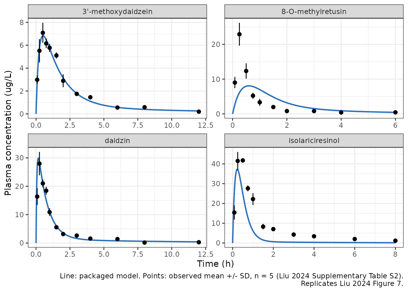
Three of the four constituents track the observations closely. 8-O-methylretusin does not, and the reason is arithmetic rather than graphical – see Assumptions and deviations.
PKNCA validation
concData <- simObs |>
  filter(!is.na(Cc)) |>
  select(id, constituent, time, Cc_ugL)

doseData <- constituents |>
  transmute(id, constituent, time = 0, dose_mgkg)

oConc <- PKNCA::PKNCAconc(
  concData, Cc_ugL ~ time | constituent + id,
  concu = "ug/L", timeu = "h"
)
oDose <- PKNCA::PKNCAdose(
  doseData, dose_mgkg ~ time | constituent + id,
  doseu = "mg/kg"
)

intervals <- constituents |>
  transmute(
    constituent, id,
    start = 0, end = tlast_h,
    cmax = TRUE, tmax = TRUE, auclast = TRUE,
    aucinf.obs = TRUE, half.life = TRUE
  )

ncaRes <- PKNCA::pk.nca(PKNCA::PKNCAdata(oConc, oDose, intervals = intervals))

simNca <- as.data.frame(ncaRes) |>
  filter(PPTESTCD %in% c("cmax", "tmax", "auclast", "aucinf.obs", "half.life")) |>
  select(constituent, PPTESTCD, PPORRES)

stopifnot(nrow(simNca) == 20L, !anyNA(simNca$PPORRES))
Comparison against the published NCA
The reference values are the statistical-moment parameters of
Supplementary Tables S4, S6, S8 and S10. These are the same numbers as
the “Val.” rows of the main article’s Table 4, which reports them in
ug/mL rather than ug/L (e.g. daidzin Cmax 0.0272 ug/mL =
27.2 ug/L vs. 27.183 ug/L in Table S8).
refNca <- tribble(
  ~constituent,          ~cmax,  ~tmax, ~auclast, ~aucinf.obs, ~half.life,
  "3'-methoxydaidzein",   7.179,  0.55,   19.127,      20.023,      2.900,
  "8-O-methylretusin",   25.268,  0.25,   15.278,      15.459,      1.067,
  "daidzin",             27.183,  0.25,   35.516,      35.920,      1.822,
  "isolariciresinol",    41.698,  0.30,   55.749,      59.323,      1.727
)

ncaTable <- nlmixr2lib::ncaComparisonTable(
  simNca, refNca,
  by = "constituent",
  units = c(cmax = "ug/L", auclast = "ug*h/L", aucinf.obs = "ug*h/L",
            tmax = "h", half.life = "h")
)
knitr::kable(ncaTable)| NCA parameter | constituent | Reference | Simulated | % diff |
|---|---|---|---|---|
| Cmax (ug/L) | 3’-methoxydaidzein | 7.18 | 6.83 | -4.9% |
| Cmax (ug/L) | 8-O-methylretusin | 25.3 | 7.95 | -68.5%* |
| Cmax (ug/L) | daidzin | 27.2 | 28.5 | +4.9% |
| Cmax (ug/L) | isolariciresinol | 41.7 | 37.1 | -11.1% |
| Tmax (h) | 3’-methoxydaidzein | 0.55 | 0.5 | -9.1% |
| Tmax (h) | 8-O-methylretusin | 0.25 | 0.5 | +100.0%* |
| Tmax (h) | daidzin | 0.25 | 0.25 | +0.0% |
| Tmax (h) | isolariciresinol | 0.3 | 0.25 | -16.7% |
| AUC0-∞ (obs) (ug*h/L) | 3’-methoxydaidzein | 20 | 19.5 | -2.5% |
| AUC0-∞ (obs) (ug*h/L) | 8-O-methylretusin | 15.5 | 17.1 | +10.7% |
| AUC0-∞ (obs) (ug*h/L) | daidzin | 35.9 | 38.8 | +8.0% |
| AUC0-∞ (obs) (ug*h/L) | isolariciresinol | 59.3 | 25.4 | -57.1%* |
| AUClast (ug*h/L) | 3’-methoxydaidzein | 19.1 | 17.5 | -8.2% |
| AUClast (ug*h/L) | 8-O-methylretusin | 15.3 | 16 | +5.0% |
| AUClast (ug*h/L) | daidzin | 35.5 | 34.8 | -1.9% |
| AUClast (ug*h/L) | isolariciresinol | 55.7 | 24.8 | -55.5%* |
| t½ (h) | 3’-methoxydaidzein | 2.9 | 5.36 | +84.9%* |
| t½ (h) | 8-O-methylretusin | 1.07 | 1.7 | +59.0%* |
| t½ (h) | daidzin | 1.82 | 6.69 | +267.1%* |
| t½ (h) | isolariciresinol | 1.73 | 3.19 | +84.5%* |
- differs from reference by more than ±20%.
The starred rows have identified causes:
-
8-O-methylretusin
cmax– the publishedV1/Fis too large to reach the observed peak at all (below). This is the one genuine model-versus-data failure. -
isolariciresinol
auclast/aucinf.obs– the publishedCL/Fis internally inconsistent with the same table’s own AUC (below). -
half.life, all four – the terminal phase is not identifiable from a profile truncated at 6-12 h, and the paper says so twice over. Liu 2024 reports two estimates of this quantity per constituent, and they disagree by an order of magnitude: the statistical-momentt1/2z(2.90, 1.07, 1.82, 1.73 h, used as the reference column above) and the compartmentalt1/2betafrom the very same fit (14.4 +/- 15.5, 35.4 +/- 39.1, 36.5 +/- 37.8 and 17.4 +/- 29.1 h – every one with an SD of the same order as its mean). The packaged models’ true beta half-lives are 7.90, 2.25, 6.80 and 3.21 h, i.e. bracketed by the paper’s own two estimates in every case. There is no model defect to fix here; the reference number is one of two irreconcilable values the source publishes for the same parameter.
Model-consistency check
For a linear model dosed into a depot with complete input, total
AUC must equal dose / (CL/F) exactly. This
checks the packaged parameters and the NCA harness against each other
rather than against the paper. It is computed on the 120 h grid so that
auclast is the entire AUC and no lambda-z extrapolation
enters – otherwise the check would pass on the strength of a correct
auclast even if the terminal slope were wrong.
oConcLong <- PKNCA::PKNCAconc(
  simLong |> select(id, constituent, time, Cc_ugL),
  Cc_ugL ~ time | constituent + id,
  concu = "ug/L", timeu = "h"
)
ncaLong <- PKNCA::pk.nca(PKNCA::PKNCAdata(
  oConcLong, oDose,
  intervals = constituents |>
    transmute(constituent, id, start = 0, end = 120, auclast = TRUE)
))

aucCheck <- as.data.frame(ncaLong) |>
  filter(PPTESTCD == "auclast") |>
  left_join(constituents, by = "constituent") |>
  left_join(
    tibble(
      constituent = names(modelNames),
      clf = vapply(uis, function(u) exp(u$theta[["lcl"]]), numeric(1))
    ),
    by = "constituent"
  ) |>
  mutate(
    analytic_ugLh = dose_mgkg / clf * 1000,
    pct_diff      = 100 * (PPORRES - analytic_ugLh) / analytic_ugLh
  )

aucCheck |>
  select(constituent, PPORRES, analytic_ugLh, pct_diff) |>
  rename(
    "Constituent" = constituent,
    "AUC(0-120 h) by PKNCA (ug*h/L)" = PPORRES,
    "Dose / (CL/F) (ug*h/L)" = analytic_ugLh,
    "% difference" = pct_diff
  ) |>
knitr::kable(digits = 4)| Constituent | AUC(0-120 h) by PKNCA (ug*h/L) | Dose / (CL/F) (ug*h/L) | % difference |
|---|---|---|---|
| 3’-methoxydaidzein | 20.4615 | 20.4620 | -0.0029 |
| 8-O-methylretusin | 17.5267 | 17.5271 | -0.0020 |
| daidzin | 39.2730 | 39.2784 | -0.0137 |
| isolariciresinol | 26.3111 | 26.3155 | -0.0169 |
Assumptions and deviations
Macro versus micro parameterisation
Supplementary Tables S3/S5/S7/S9 print two complete
parameterisations of the same two-compartment model: a macro
set (V1/F, CL/F) and a micro-constant set
(K10, K12, K21). Because DAS 2.0
fitted each rat separately and the table reports arithmetic means, the
two sets cannot be mutually consistent –
mean(K10) * mean(V1/F) is not mean(CL/F). The
packaged models use the macro set (cl =
CL/F, vc = V1/F), which is the
canonical nlmixr2lib parameterisation, with K12 and
K21 taken directly because DAS 2.0 reports no
V2/F or Q/F.
The choice was made on the numbers, not by preference. The table
below is the worst fold-error across Cmax,
Tmax, AUC(0-inf) and terminal half-life when
each candidate clearance is substituted into the same structure,
together with the log-scale R-squared of the predicted curve against the
45 observed means:
| Constituent |
K10 * V1/F (micro) |
CL/F (macro, used) |
CLz/F (statistical moment) |
|---|---|---|---|
| 3’-methoxydaidzein | 6.077 – worst FE 2.72, R2 0.978 | 6.06 – worst FE 2.72, R2 0.978 | 6.197 – worst FE 2.70, R2 0.978 |
| 8-O-methylretusin | 80.34 – worst FE 7.87, R2 0.891 | 12.552 – worst FE 3.13, R2 0.604 | 14.250 – worst FE 3.27, R2 0.644 |
| daidzin | 36.58 – worst FE 3.70, R2 0.907 | 35.643 – worst FE 3.73, R2 0.908 | 39.111 – worst FE 3.62, R2 0.904 |
| isolariciresinol | 222.15 – worst FE 5.03, R2 0.820 | 99.561 – worst FE 2.25, R2 0.909 | 44.282 – worst FE 2.18, R2 0.966 |
For 3’-methoxydaidzein and daidzin the three candidates are
interchangeable (K10 * V1/F agrees with the published
CL/F to 0.3% and 2.6%). For the other two they are not, and
the published SDs explain why: 8-O-methylretusin has
K10 = 6.671 (SD 10.483) and V1/F = 12.043 (SD
17.445); isolariciresinol has K10 = 7.512 (SD 14.088) and
CL/F = 99.561 (SD 130.836). An arithmetic mean whose SD
exceeds it describes no animal in the study.
Errata and defects in the source
-
8-O-methylretusin
V1/Fis infeasible against the paper’s own data. With a dose of 0.22 mg/kg andV1/F= 12.043 L/kg, the highest attainable plasma concentration is 0.22 / 12.043 = 18.3 ug/L even with instantaneous, complete absorption and no elimination. Supplementary Table S2 reports an observed mean of 22.891 ug/L at 0.25 h, and Table S6 reportsCmax= 25.268 ug/L. No choice ofKa,K12orK21can repair this; the volume itself is too large. The publishedKacompounds the problem: 2.056 1/h with a reported absorption half-life of 20.246 h (SD 33.118) cannot produce the observed 0.25 hTmax. The parameters are encoded as published rather than adjusted, so this model reproduces the publication, not the data. -
Isolariciresinol
CL/Fis irreconcilable with its own table. Table S9 givesCL/F= 99.561 L/h/kg andAUC(0-inf)= 52.808 ugh/L in the same column;dose / (CL/F)is 26.3 ugh/L, a two-fold internal contradiction. The statistical-momentCLz/Fof 44.282 L/h/kg (SD 2.557) in Table S10 reproduces the observed AUC exactly.CL/Fis retained for consistency with the other three models and because it is part of the fitted compartmental model; users wanting to match the observed exposure should substitutelcl <- log(44.282). - Duplicated observations. In Supplementary Table S2, 8-O-methylretusin has identical mean and SD at 2 h and 3 h (0.809 +/- 0.103). This is almost certainly a transcription duplicate; it is reproduced verbatim above.
- Compound-name typo in the main article. The main text spells constituent 1 “3’-methoxydadizein” throughout (transposed letters). The supplement and the chemical structure in Figure 1 both give “3’-methoxydaidzein”, which is the spelling used here.
- Daidzin dose. The main text gives the doubled daidzin dose as 1.42 mg/kg (Section 2.2) while Supplementary Table S2 heads the same experiment “1.4 mg/kg”. The supplement value is used because the compartmental parameters were fitted to that dataset; the 1.4% difference propagates linearly to AUC.
What is not extracted
The GastroPlus PBPK model. Liu 2024 Equation (1) prints the perfusion-limited ODE system for lung, liver (with a Michaelis-Menten hepatic term), kidney, heart, muscle, spleen, brain, rest-of-body, artery and vein, and Table 2 gives 13 rat tissue partition coefficients. That is not enough to solve it. The paper never prints:
- any tissue volume
Vior blood flowQi– these are GastroPlus built-in rat physiology; - any absorption model – the GI compartment appears in the liver
equation as
QGI * CGI / kGIbut has no differential equation, no partition coefficient in Table 2 and no ACAT parameters; - the enterohepatic recirculation settings, even though Section 3 states the GastroPlus enterohepatic module was enabled to fit the secondary peaks at 3 h and 6 h;
- the renal clearance
Cl'Kseparately from totalCL; - the CYP abundance scalars needed to interpret
Vmaxreported in nM/min/nM; - human tissue partition coefficients (Table 2 is rat only).
Because PBPK models in this library are built only from the sources that were available, these gaps are not filled from GastroPlus defaults or class-typical values, so the PBPK layer is out of scope.
The human extrapolation. Table 5 reports predicted
human Cmax, Tmax and AUC. Equation (3) gives
the single-species allometric scaling used for clearance
(CLu,human = CLu,rat * (70 / 0.25)^0.75), but the human
volume came from Equation (4) applied to human partition
coefficients and tissue volumes that are never reported, so the human
model is not reproducible either.
Multiple-dose and dose-escalation predictions (Figures 5 and 6) are GastroPlus PBPK outputs and inherit the same gaps.
Other assumptions
- Concentrations are simulated as typical values; no residual error is
added (
addSdisfixed(0)), because Liu 2024 reports no residual-error model. - No between-subject variability is encoded. The SDs in Tables S3-S10
are arithmetic SDs of five individually fitted rats, not estimated
variance components, and for several parameters they exceed the mean, so
they cannot be read as log-normal
omegavalues. They are recorded in theini()comments. -
CL/FandV1/Fare apparent: the route is oral and Liu 2024 determined no bioavailability. Doses are per kg body weight, so volumes are L/kg and clearances L/h/kg. -
The peripheral transfer is stored as
q/vp, not as the publishedK12/K21. This is a deliberate safety choice, not a preference.rxode2::rxSolve()withuseLinCmt = TRUErewrites a recognisably linear system into a closed form; with ak12/k21parameterisation it matches onlyclandvc, converts the model to a one-compartment solution and silently discardsperipheral1. The profile then decays withkelinstead of beta – 1.47 h instead of 7.90 h for 3’-methoxydaidzein – while total AUC stays exactlydose/(CL/F), so an exposure check does not reveal it. Withq/vpthe conversion is correct and the default call is safe.Q/F = K12 * V1/FandV2/F = Q/F / K21are exact, and the arithmetic is written out in eachini()so the published micro-constants remain visible. The simulation chunk asserts the simulated terminal slope equals the analytic beta root, which would fail if a future edit reintroduced the collapse.