Model and source
- Citation: Boer H, Proost JH, Nuver J, Bunskoek S, Gietema JQ, Geubels BM, Altena R, Zwart N, Oosting SF, Vonk JM, Lefrandt JD, Uges DRA, Meijer C, de Vries EGE, Gietema JA. Long-term exposure to circulating platinum is associated with late effects of treatment in testicular cancer survivors. Ann Oncol. 2015;26(11):2305-2310. doi:10.1093/annonc/mdv369
- Description: Two-compartment population PK model for long-term circulating platinum (Pt) decay after cisplatin-based chemotherapy in adult testicular cancer survivors followed 1-13 years post-treatment (Boer 2015). Dose is the cumulative cisplatin dose expressed as elemental Pt in mg (multiply cumulative cisplatin in mg by 0.6502, the Pt/cisplatin mass ratio 195.08/300.05). An apparent bioavailability F1 (fdepot) accounts for the fraction of the administered Pt remaining in the body after the rapid pre-measurement urinary-excretion phase. Pt is assumed to be cleared solely via urine.
- Article: https://doi.org/10.1093/annonc/mdv369 (Open Access, CC-BY-NC; PMC4621032)
- Supplementary materials (Tables S1-S6 and Figures S1-S2): obtained
via the Europe PMC supplementary-files endpoint
https://www.ebi.ac.uk/europepmc/webservices/rest/PMC4621032/supplementaryFiles.
Boer et al. modelled the slow decay of circulating platinum (Pt) in
serum of 96-99 testicular-cancer survivors followed 1-13 years after
curative cisplatin-based chemotherapy. A two-compartment open model with
apparent bioavailability F1 was fit to 240 serum Pt
concentrations and 91 spot 24-h urinary excretion rates simultaneously.
The model carries the fraction of administered Pt still circulating
after the rapid post-treatment urinary phase; the published terminal
half-life of 3.7 years (range 2.5-5.2) reflects slow release from a
peripheral tissue reservoir.
Population
The model was developed in 99 Dutch men (UMC Groningen single-centre) treated for non-seminomatous testicular cancer with cisplatin-based chemotherapy between 1988 and 2000. Median age at start of chemotherapy was 29 years (range 17-53); median age at follow-up assessment was 39 years (range 23-64). Disease stage was Royal Marsden II/III/IV = 53%/5%/42% and IGCCCG risk good/intermediate/poor = 56%/34%/9%. Chemotherapy regimens were 4xBEP (33%), 4xEP (8%), 3xBEP/1xEP (52%), and other cisplatin-based combinations (6%); median cumulative cisplatin dose 809 mg (range 554-1713; equivalently 400 mg/m^2, range 275-800). 240 serum Pt samples and 91 24-h urine samples were collected at follow-up visits between 0.9 and 13.2 years post-start-of-chemotherapy. Baseline demographics are reported in Boer 2015 Table 1.
The same information is available programmatically via
rxode2::rxode(readModelDb("Boer_2015_cisplatin"))$population.
Source trace
Per-parameter origins are recorded in the in-file comments of
inst/modeldb/specificDrugs/Boer_2015_cisplatin.R. The table
below collects them in one place for review.
| Equation / parameter | Value | Source location |
|---|---|---|
Two-compartment structural form
Ct = F1 * Dose / V1 * (C1 * exp(-lambda1*t) + C2 * exp(-lambda2*t))
|
– | Boer 2015, “population PK model” section (page 2307) |
CL |
0.0220 L/day (95% CI 0.0197-0.0246) | Suppl Table S1 |
V1 (vc) |
6.61 L (95% CI 5.20-8.03) | Suppl Table S1 |
Q |
0.00531 L/day (95% CI 0.00461-0.00611) | Suppl Table S1 |
V2 (vp) |
8.05 L (95% CI 6.55-10.17) | Suppl Table S1 |
F1 (fdepot) |
0.000158 (95% CI 0.000137-0.000188) | Suppl Table S1 |
| IIV CL = 13% | omega^2 = 0.01676 | Suppl Table S1 |
| IIV V2 = 22% | omega^2 = 0.04728 | Suppl Table S1 |
| IIV F1 = 17% | omega^2 = 0.02847 | Suppl Table S1 |
| Proportional residual error | 34% | Boer 2015 Results, “population PK model” section (page 2307) |
| Mean terminal T1/2 = 3.7 yr (range 2.5-5.2) | derived | Boer 2015 Results, “population PK model” section |
| Median Pt at 1, 3, 5, 10 yr | 2876 / 391 / 197 / 74 ng/L | Suppl Table S2 |
| Median Pt AUC(1-3 yr) | 27.9 ug/L * month (range 16.1-56.7) | Suppl Table S2 |
Virtual cohort
Original observed data are not publicly available. Two virtual cohorts are constructed:
- Typical-value cohort: a single subject dosed at the cohort median cumulative Pt dose, for replicating the typical-decay curve that Boer 2015 Figure 1 shows as the central line.
- Stochastic cohort: 200 virtual subjects with cumulative Pt doses sampled from the paper’s reported cisplatin-dose range (554-1713 mg cisplatin = 360-1114 mg Pt), used for PKNCA validation and to bracket the population-level decay range.
The dose-input column in the model is elemental platinum in mg, which is the cumulative cisplatin mg dose multiplied by the Pt-to- cisplatin mass ratio 195.08 / 300.05 = 0.6502 (Pt atomic weight / cisplatin formula weight). The median 809 mg cisplatin therefore corresponds to a dose-input of 526 mg Pt.
set.seed(20250603)

Pt_per_cisplatin <- 195.08 / 300.05  # = 0.6502

# Cumulative cisplatin in mg (range 554-1713, median 809 per Boer 2015
# Table 1). Sample from a log-normal centred on the published median
# with sigma_log chosen so the 95% range brackets the observed range;
# truncate to the reported min/max.
n_subj <- 200L
cisplatin_raw <- stats::rlnorm(n_subj, meanlog = log(809), sdlog = 0.25)
cisplatin_mg  <- pmin(pmax(cisplatin_raw, 554), 1713)
Pt_dose_mg    <- cisplatin_mg * Pt_per_cisplatin

# Observation grid: weekly samples between 0 and 13.5 years
obs_times_d <- seq(0, 13.5 * 365.25, by = 7)

make_cohort <- function(ids, doses_mg, obs_times_d, cohort_label) {
  dose_rows <- data.frame(
    id   = ids,
    time = 0,
    amt  = doses_mg,
    cmt  = "central",
    evid = 1L,
    Cc   = NA_real_
  )
  obs_rows <- expand.grid(id = ids, time = obs_times_d) |>
    transform(amt = NA_real_, cmt = "central", evid = 0L, Cc = NA_real_)
  out <- rbind(dose_rows, obs_rows)
  out <- out[order(out$id, out$time, -out$evid), ]
  out$cohort <- cohort_label
  out
}

# Stochastic cohort
events_stoch <- make_cohort(
  ids        = seq_len(n_subj),
  doses_mg   = Pt_dose_mg,
  obs_times_d = obs_times_d,
  cohort_label = "stochastic"
)

# Typical-value cohort (single virtual subject, median dose)
typical_dose_mg <- 809 * Pt_per_cisplatin
events_typical <- make_cohort(
  ids        = n_subj + 1L,
  doses_mg   = typical_dose_mg,
  obs_times_d = obs_times_d,
  cohort_label = "typical"
)

stopifnot(!anyDuplicated(unique(events_stoch[, c("id", "time", "evid")])))
stopifnot(!anyDuplicated(unique(events_typical[, c("id", "time", "evid")])))
Simulation
mod <- boer_mod

sim_stoch <- rxode2::rxSolve(
  mod, events = events_stoch,
  keep = c("cohort")
) |> as.data.frame()

sim_typical <- rxode2::rxSolve(
  rxode2::zeroRe(mod), events = events_typical,
  keep = c("cohort")
) |> as.data.frame()
#> ℹ omega/sigma items treated as zero: 'etalcl', 'etalvp', 'etalfdepot'
Replicate published figures
Figure 1 – median + extremes of circulating Pt over 1-13 years
# Boer 2015 Figure 1 shows the predicted median curve plus the highest
# and lowest predicted decay across the cohort, on a linear y-scale
# (ug/L) over years 1-13.
sim_summary <- sim_stoch |>
  dplyr::filter(time > 0) |>
  dplyr::mutate(year = time / 365.25) |>
  dplyr::group_by(year) |>
  dplyr::summarise(
    median = stats::median(Cc, na.rm = TRUE),
    high   = max(Cc, na.rm = TRUE),
    low    = min(Cc, na.rm = TRUE),
    .groups = "drop"
  )

ggplot(sim_summary, aes(x = year)) +
  geom_line(aes(y = median), linewidth = 1) +
  geom_line(aes(y = high),   linetype = "dashed") +
  geom_line(aes(y = low),    linetype = "dashed") +
  scale_x_continuous(limits = c(1, 13), breaks = seq(1, 13, by = 2)) +
  labs(
    x = "Years after start of chemotherapy",
    y = expression(paste("Serum platinum (", mu, "g/L)")),
    title = "Figure 1 -- typical, maximum and minimum predicted Pt decay",
    caption = "Replicates Figure 1 of Boer 2015 (median + highest/lowest predicted decay)."
  )
#> Warning: Removed 78 rows containing missing values or values outside the scale range
#> (`geom_line()`).
#> Removed 78 rows containing missing values or values outside the scale range
#> (`geom_line()`).
#> Removed 78 rows containing missing values or values outside the scale range
#> (`geom_line()`).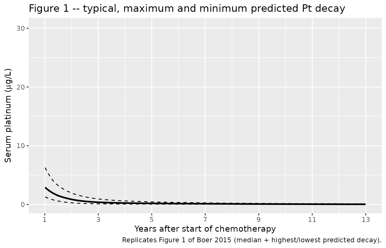
Comparison against published predictions (Supplementary Table S2)
Boer 2015 Supplementary Table S2 reports the median predicted Pt concentration at fixed time points after chemotherapy and the median AUC over years 1-3.
time_points_yr <- c(1, 3, 5, 10)
sim_at_pts <- sim_stoch |>
  dplyr::filter(time > 0) |>
  dplyr::mutate(year = time / 365.25) |>
  dplyr::group_by(id) |>
  dplyr::summarise(
    `1`  = stats::approx(year, Cc, xout = 1)$y,
    `3`  = stats::approx(year, Cc, xout = 3)$y,
    `5`  = stats::approx(year, Cc, xout = 5)$y,
    `10` = stats::approx(year, Cc, xout = 10)$y,
    .groups = "drop"
  ) |>
  tidyr::pivot_longer(-id, names_to = "year", values_to = "Cc_ug_L") |>
  dplyr::group_by(year) |>
  dplyr::summarise(
    median_ng_L = stats::median(Cc_ug_L, na.rm = TRUE) * 1000,
    min_ng_L    = min(Cc_ug_L, na.rm = TRUE)            * 1000,
    max_ng_L    = max(Cc_ug_L, na.rm = TRUE)            * 1000,
    .groups = "drop"
  ) |>
  dplyr::mutate(year_num = as.integer(year)) |>
  dplyr::arrange(year_num)

published <- tibble::tribble(
  ~year_num, ~published_median, ~published_min, ~published_max,
  1L,        2876,              1723,           5519,
  3L,        391,               225,            939,
  5L,        197,               113,            453,
  10L,       74,                30,             165
)

comparison_pt <- sim_at_pts |>
  dplyr::left_join(published, by = "year_num") |>
  dplyr::transmute(
    `Time (years)`            = year_num,
    `Published median (ng/L)` = published_median,
    `Simulated median (ng/L)` = round(median_ng_L, 0),
    `Published range (ng/L)`  = sprintf("%d -- %d", published_min, published_max),
    `Simulated range (ng/L)`  = sprintf("%d -- %d", round(min_ng_L, 0), round(max_ng_L, 0))
  )
knitr::kable(comparison_pt,
caption = "Concentration comparison vs Boer 2015 Suppl Table S2 (median, range across cohort).")| Time (years) | Published median (ng/L) | Simulated median (ng/L) | Published range (ng/L) | Simulated range (ng/L) |
|---|---|---|---|---|
| 1 | 2876 | 2970 | 1723 – 5519 | 1333 – 6424 |
| 3 | 391 | 389 | 225 – 939 | 118 – 954 |
| 5 | 197 | 198 | 113 – 453 | 67 – 455 |
| 10 | 74 | 76 | 30 – 165 | 25 – 170 |
auc_1_3 <- sim_stoch |>
  dplyr::filter(time >= 365.25, time <= 3 * 365.25) |>
  dplyr::arrange(id, time) |>
  dplyr::group_by(id) |>
  dplyr::summarise(
    auc_ug_L_day = sum(diff(time) *
                       (utils::head(Cc, -1) + utils::tail(Cc, -1)) / 2,
                       na.rm = TRUE),
    .groups = "drop"
  ) |>
  dplyr::mutate(auc_ug_L_month = auc_ug_L_day * 12 / 365.25)

cat(sprintf(
  "Simulated AUC(1-3 years): median %.1f ug/L*month (range %.1f -- %.1f)\n",
  stats::median(auc_1_3$auc_ug_L_month),
  min(auc_1_3$auc_ug_L_month),
  max(auc_1_3$auc_ug_L_month)
))
#> Simulated AUC(1-3 years): median 26.3 ug/L*month (range 9.9 -- 56.5)
cat("Boer 2015 Suppl Table S2: median 27.9 ug/L*month (range 16.1 -- 56.7)\n")
#> Boer 2015 Suppl Table S2: median 27.9 ug/L*month (range 16.1 -- 56.7)
PKNCA validation
NCA was not reported in the paper, but two derived quantities are:
the terminal half-life (T1/2 = 3.7 years, range 2.5-5.2
across subjects, Boer 2015 Results) and the AUC(1-3 years). Run PKNCA on
the stochastic cohort to compute terminal half-life per subject and
AUC(0-Inf), and compare the terminal half-life distribution against the
paper’s reported range.
The PKNCA dose unit is the model dose in mg (elemental Pt). Time is in days.
sim_nca <- sim_stoch |>
  dplyr::filter(!is.na(Cc), time > 0) |>
  dplyr::select(id, time, Cc, cohort)

conc_obj <- PKNCA::PKNCAconc(sim_nca, Cc ~ time | cohort + id)

dose_df <- events_stoch |>
  dplyr::filter(evid == 1) |>
  dplyr::select(id, time, amt, cohort)

dose_obj <- PKNCA::PKNCAdose(dose_df, amt ~ time | cohort + id)

intervals <- data.frame(
  start      = 0,
  end        = Inf,
  aucinf.obs = TRUE,
  half.life  = TRUE
)

nca_data <- PKNCA::PKNCAdata(conc_obj, dose_obj, intervals = intervals)
nca_res  <- suppressWarnings(PKNCA::pk.nca(nca_data))

nca_indiv <- as.data.frame(nca_res$result)

half_life_d <- nca_indiv |>
  dplyr::filter(PPTESTCD == "half.life") |>
  dplyr::pull(PPORRES)
half_life_yr <- half_life_d / 365.25

cat(sprintf(
  "Simulated terminal T1/2: median %.2f yr (range %.2f -- %.2f, n = %d)\n",
  stats::median(half_life_yr, na.rm = TRUE),
  stats::quantile(half_life_yr, 0.025, na.rm = TRUE),
  stats::quantile(half_life_yr, 0.975, na.rm = TRUE),
  sum(!is.na(half_life_yr))
))
#> Simulated terminal T1/2: median 3.70 yr (range 2.50 -- 5.58, n = 200)
cat("Boer 2015: mean terminal T1/2 = 3.7 yr (range 2.5 -- 5.2)\n")
#> Boer 2015: mean terminal T1/2 = 3.7 yr (range 2.5 -- 5.2)
nca_summary <- summary(nca_res)
knitr::kable(nca_summary,
caption = "PKNCA: simulated population NCA parameters (single cohort).")| start | end | cohort | N | half.life | aucinf.obs |
|---|---|---|---|---|---|
| 0 | Inf | stochastic | 200 | 1390 [280] | NC |
Assumptions and deviations
-
Dose units. The model accepts elemental Pt in mg.
To dose with cumulative cisplatin in mg, multiply by
195.08 / 300.05 = 0.6502(Pt atomic weight / cisplatin formula weight). This matches the paper’s note “cumulative cisplatin dose (mg/m^2, converted to amount Pt in mg)”. -
Initial time point. The popPK analysis was
restricted to the fraction of Pt remaining in the body after the rapid
pre-measurement urinary phase (Boer 2015 Methods, “population PK
analysis”). The model’s
t = 0is therefore the end of cisplatin chemotherapy (the 9-12 week treatment window is treated as negligible relative to the 1-13 year follow-up), andF1(fdepot) captures the small fraction (~0.016%) of administered Pt that survives the initial urinary-excretion phase to enter the long-term distribution. -
No covariates. Boer 2015 tested age, weight,
height, BMI and body surface area in covariate screening and did not
retain any in the final model (Results, “population PK model”). The
model has no covariate-effect parameters. Three demographic covariates
were recorded in the source dataset and screened (
AGE,WT,HT); they are kept incovariatesDataExcludedrather thancovariateDataso they are not flagged as declared-but-unused bycheckModelConventions(). -
Residual error magnitude. Suppl Table S1 does not
list a numeric SD for the residual error; the main-text statement
“Proportional residual error in the final model was 34%” is interpreted
as the CV of a proportional error and encoded as
propSd <- 0.34. -
Pt clearance pathway. The model assumes Pt is
cleared solely via urinary excretion (Boer 2015 Methods, “population PK
analysis”); the urinary excretion rate in the source dataset was fit
simultaneously with serum Pt as
CL x Cc. The packaged nlmixr2lib model exposes the serum compartment only; users needing the urinary excretion rate can compute it post hoc ascl * Cc * 1e-3(mg/day, with Cc in ug/L converted back to mg/L). -
Bioavailability compartment. Apparent F1 is applied
via
f(central) <- fdepotbecause the source structural model is an IV bolus with no absorption phase. The canonicallfdepot/fdepotparameter name is retained even though nodepotcompartment is declared, to match the nlmixr2lib bioavailability convention andcheckModelConventions()expectations.