SCR430 time-dependent pharmacokinetics in rats (Kim 2022)

Model and source

• Citation: Kim M-C, Lee Y-J. Analysis of Time-Dependent Pharmacokinetics Using In Vitro-In Vivo Extrapolation and Physiologically Based Pharmacokinetic Modeling. Pharmaceutics. 2022;14(12):2562. doi:10.3390/pharmaceutics14122562.
• Article: https://doi.org/10.3390/pharmaceutics14122562 (open access)

SCR430 is an investigational sorafenib derivative. In rats, 14 days of oral SCR430 at 30 mg/kg/day lowered the exposure to a later 3 mg/kg intravenous dose about 4.4-fold. Kim and Lee isolated hepatocytes from untreated and pretreated rats. They found that hepatic uptake, not metabolism, had increased. They then built a minimal PBPK (mPBPK) model in Berkeley Madonna. The model explains the plasma and liver profiles of both groups by swapping in each group’s hepatocyte-derived inputs. The model has one structure and two parameter sets, packaged as two files:

• Kim_2022_SCR430_rat_control_pbpk: Preclinical (rat). PBPK (minimal, IVIVE-based, Berkeley Madonna). SCR430 (investigational sorafenib derivative) in untreated (control) female Sprague-Dawley rats after a 3 mg/kg intravenous bolus. A systemic blood compartment exchanges with a single-adjustment compartment by first-order rate constants, and the liver is a five-unit tandem (dispersion-model emulation) of extracellular and hepatocellular spaces linked in series by hepatic blood flow. Hepatocyte entry is active uptake plus passive diffusion acting on the unbound blood concentration; passive efflux and intrinsic metabolic clearance act on the unbound hepatocellular concentration. The hepatic uptake, diffusion, metabolism and intracellular-binding inputs come from hepatocytes isolated from control rats (IVIVE Method 2) and carry the source paper’s empirical 1.6-fold scaling factor on the permeability clearances; the compartment volume and exchange rate constants were fitted to the plasma profile. Between-animal variability on the four hepatic inputs is the source paper’s lognormal Monte Carlo distribution. Companion model: Kim_2022_SCR430_rat_repeatedDosing_pbpk (after 14 days of oral SCR430, with induced hepatic uptake).
• Kim_2022_SCR430_rat_repeatedDosing_pbpk: Preclinical (rat). PBPK (minimal, IVIVE-based, Berkeley Madonna). SCR430 (investigational sorafenib derivative) in female Sprague-Dawley rats pretreated with oral SCR430 30 mg/kg once daily for 14 days (repeated-dosing group, auto-induced hepatic uptake), after a 2-day washout and a 3 mg/kg intravenous bolus. A systemic blood compartment exchanges with a single-adjustment compartment by first-order rate constants, and the liver is a five-unit tandem (dispersion-model emulation) of extracellular and hepatocellular spaces linked in series by hepatic blood flow. Hepatocyte entry is active uptake plus passive diffusion acting on the unbound blood concentration; passive efflux and intrinsic metabolic clearance act on the unbound hepatocellular concentration. The hepatic uptake, diffusion, metabolism and intracellular-binding inputs come from hepatocytes isolated from repeated-dosing rats (IVIVE Method 2) and carry the source paper’s empirical 1.6-fold scaling factor on the permeability clearances; the compartment volume and exchange rate constants are those fitted for the control group (‘Equal to Control’). Between-animal variability on the four hepatic inputs is the source paper’s lognormal Monte Carlo distribution. Companion model: Kim_2022_SCR430_rat_control_pbpk (untreated rats).

The structure is a systemic blood compartment, a “single-adjustment” compartment exchanging with it by first-order rate constants (k12 = paper kin, k21 = paper kout), and a liver of five extracellular units (is_liver1..is_liver5) in series along hepatic blood flow. Each unit has a hepatocellular unit (int_liver1..int_liver5) attached (paper Figure 7, Appendix A.2 Eqs. A1 to A3). Unbound blood drug enters hepatocytes by active uptake plus passive diffusion. Unbound hepatocellular drug leaves by passive efflux and intrinsic metabolism.

Population

Female Sprague-Dawley rats (8 weeks old, 190 to 205 g; Dahan Bio Link, Republic of Korea) were split into three groups of six (paper Figure 1, Section 2.2): untreated control, vehicle only for 14 days, and SCR430 30 mg/kg/day orally for 14 days (repeated dosing). After a 2-day washout each rat received SCR430 3 mg/kg intravenously; plasma was sampled to 10 h, and the liver was excised at 10 h. The vehicle group did not differ from the control group (Table 1), and the mPBPK model was built for the control and repeated-dosing groups only. The hepatic inputs come from hepatocytes isolated from rats in each group. The model is not a population fit, and only the systemic volume and the two single-adjustment rate constants were fitted to plasma data.

str(readModelDb("Kim_2022_SCR430_rat_control_pbpk")()$population)
#> List of 10
#>  $ species       : chr "rat (female Sprague-Dawley)"
#>  $ n_subjects    : int 6
#>  $ n_studies     : int 1
#>  $ age_range     : chr "8 weeks"
#>  $ weight_range  : chr "190-205 g"
#>  $ sex_female_pct: num 100
#>  $ disease_state : chr "Healthy, untreated (control) rats: no vehicle and no SCR430 before the pharmacokinetic study (source paper Figure 1, red arm)."
#>  $ dose_range    : chr "SCR430 3 mg/kg single intravenous bolus in 50% Solutol HS15 / 50% polyethylene glycol 400; plasma sampled to 10"| __truncated__
#>  $ regions       : chr "Republic of Korea (Kyung Hee University)"
#>  $ notes         : chr "n = 6 rats per group for the intravenous study (Table 1). The model itself was not fitted to individual animals"| __truncated__

Source trace

Every ini() value carries an in-file source comment; the table collects them. “Median” rows are derived from the Table 3 (mean, SD) pairs by the paper’s own Eq. 17 (see the Assumptions section).

Parameter	Control	Repeated dosing	Source
vc systemic blood volume (L/kg)	0.018	0.018	Table 3 ‘Central’, fitted (‘Equal to Control’)
k12 = kin (1/h)	2.7	2.7	Table 3, fitted
k21 = kout (1/h)	1.0	1.0	Table 3, fitted
q_liver Qh (L/h/kg)	3.69	3.69	Table 3; Section 2.7
v_is_liver extracellular space (L/kg)	0.01	0.01	Table 3
v_int_liver hepatocytes (L/kg)	0.027	0.027	Table 3 (sums with the above to Liver 0.037)
fup	0.0078	0.0081	Table 1 fu,p
bpr Rb	3.95	4.53	Table 1 Rb
PSinf,act (L/h/kg), mean (SD)	2.5 (0.8)	9.2 (0.6)	Table 3
PSdiff (L/h/kg), mean (SD)	0.3 (0.09)	0.86 (0.4)	Table 3
CLint,met (L/h/kg), mean (SD)	9.8 (1.0)	12.3 (0.08)	Table 3
fu,hepa, mean (SD)	0.004 (0.002)	0.01 (0.008)	Table 3; Table 1
sf_ps scaling factor on PSinf,act and PSdiff	1.6	1.6	Section 3.7
l<param> typical value	ln(mean) - 0.5 ln(1 + CV^2)	same	Section 2.11 Eq. 17
etal<param> variance	ln(1 + CV^2)	same	Section 2.11 Eq. 18
Extracellular units d/dt(is_liver<i>)			Appendix A.2 Eqs. A1, A2
Hepatocellular units d/dt(int_liver<i>)			Appendix A.2 Eq. A3
Systemic / single-adjustment d/dt(central), d/dt(peripheral1)			Figure 7 schematic
Cc = systemic blood / Rb			Sections 2.9, 3.1 (see Assumptions)
Cliver = mean hepatocellular concentration			Figure 8c/d (see Assumptions)

mod_ctl <- readModelDb("Kim_2022_SCR430_rat_control_pbpk")
mod_rep <- readModelDb("Kim_2022_SCR430_rat_repeatedDosing_pbpk")
ini_ctl <- rxode2::rxode(mod_ctl)$iniDf
ini_rep <- rxode2::rxode(mod_rep)$iniDf
est <- function(ini, nm) ini$est[ini$name == nm]

IVIVE arithmetic (Table 2, Method 2)

The paper scales the hepatocyte uptake clearance (uL/min per 10^6 cells) to the whole animal with 108 x 10^6 cells/g liver and 36 g liver/kg (Section 2.5). Table 3 splits the resulting in vivo PSinf into its active and passive parts, before the 1.6-fold factor is applied:

psf <- 108 * 36 # 10^6 cells per kg body weight
ivive <- tibble(
  group = c("Control", "Repeated dosing"),
  ps_inf_hep = c(11.9, 43.2), # Table 2, uL/min per 10^6 cells
  table2_ps_inf = c(46.2, 168.0), # Table 2, mL/min/kg
  table3_sum = c(2.5 + 0.3, 9.2 + 0.86) # Table 3 PSinf,act + PSdiff, L/h/kg
) |>
  mutate(
    scaled_ps_inf = ps_inf_hep * psf / 1000, # mL/min/kg
    table3_sum_mL_min_kg = table3_sum * 1000 / 60
  )
knitr::kable(ivive, digits = 1)

group	ps_inf_hep	table2_ps_inf	table3_sum	scaled_ps_inf	table3_sum_mL_min_kg
Control	11.9	46.2	2.8	46.3	46.7
Repeated dosing	43.2	168.0	10.1	168.0	167.7

stopifnot(
  all(abs(ivive$scaled_ps_inf / ivive$table2_ps_inf - 1) < 0.01),
  all(abs(ivive$table3_sum_mL_min_kg / ivive$table2_ps_inf - 1) < 0.02)
)

The Table 3 sums reproduce the unscaled Method 2 PSinf in both groups. That is why the model applies sf_ps = 1.6 on top of the Table 3 values rather than treating the factor as already folded in.

Typical-value simulation and clearance check

The tandem liver is linear, so its plasma clearance has a closed form. Each of the five units extracts E = u / (Qh + u) of the blood passing through, where u is the unit’s share of the unbound-blood intrinsic clearance, fub * CLint,all / 5, and CLint,all = PSupt * CLint,met / (PSeff + CLint,met) (paper Eq. 6). Blood clearance is Qh * (1 - (1 - E)^5); plasma clearance is that times Rb. The integrated model must give the same number.

grid <- sort(unique(c(seq(0, 10, by = 0.05), seq(10, 96, by = 0.5))))
make_events <- function(group, n, id_offset = 0L) {
  rxode2::et(amt = 3, cmt = "central") |>
    rxode2::et(grid, cmt = "central") |>
    as.data.frame() |>
    # Two `~` endpoints (Cc, Cliver): observation rows carry dvid = 1; the
    # forward solve still returns both concentration columns.
    mutate(dvid = ifelse(evid == 0, 1L, NA_integer_)) |>
    tidyr::crossing(id = id_offset + seq_len(n)) |>
    select(-any_of("ID")) |>
    relocate(id) |>
    arrange(id, time, desc(evid)) |>
    mutate(group = group)
}
ev_typ_ctl <- make_events("Control", 1L)
ev_typ_rep <- make_events("Repeated dosing", 1L, id_offset = 1L)

typ <- bind_rows(
  as.data.frame(rxode2::rxSolve(mod_ctl, ev_typ_ctl, omega = NA, keep = "group")),
  as.data.frame(rxode2::rxSolve(mod_rep, ev_typ_rep, omega = NA, keep = "group"))
)

closed_form_cl <- function(ini) {
  fub <- est(ini, "fup") / est(ini, "bpr")
  sf <- est(ini, "sf_ps")
  ps_upt <- sf * (exp(est(ini, "lps_inf_act")) + exp(est(ini, "lps_dif")))
  ps_eff <- sf * exp(est(ini, "lps_dif"))
  clm <- exp(est(ini, "lcl_int_met"))
  clint_all <- ps_upt * clm / (ps_eff + clm)
  qh <- est(ini, "q_liver")
  u <- fub * clint_all / 5
  e_unit <- u / (qh + u)
  qh * (1 - (1 - e_unit)^5) * est(ini, "bpr") * 1000 # mL/h/kg, plasma
}

auc_typ <- typ |>
  group_by(group) |>
  summarise(
    auc = sum(diff(time) * (head(Cc, -1) + tail(Cc, -1)) / 2),
    c_last = last(Cc),
    .groups = "drop"
  ) |>
  mutate(
    cl_sim = 3 / auc * 1000, # mL/h/kg
    cl_closed = c(closed_form_cl(ini_ctl), closed_form_cl(ini_rep)),
    cl_observed = c(30.02, 137.9) # Table 1
  )
knitr::kable(auc_typ, digits = 3)

group	auc	c_last	cl_sim	cl_closed	cl_observed
Control	94.830	0.001	31.636	31.760	30.02
Repeated dosing	26.036	0.000	115.225	116.706	137.90

stopifnot(
  # Same parameters on both sides; the gap is trapezoid error and the
  # unintegrated tail beyond 96 h only.
  all(abs(auc_typ$cl_sim / auc_typ$cl_closed - 1) < 0.02)
)

At the median inputs the model’s plasma clearance is about 32 mL/h/kg in the control group (observed 30.0) and about 115 mL/h/kg after repeated dosing (observed 137.9). This reproduces the 4- to 5-fold induction of clearance that the paper attributes to hepatic uptake.

Monte Carlo simulation (Figure 8)

The paper drew 1000 virtual rats per group from lognormal distributions on PSinf,act, PSdiff, CLint,met and fu,hepa (Section 2.11). Here 200 per group are drawn from the same distributions through the models’ etas.

rxode2::rxSetSeed(20221122)
n_mc <- 200L
fig_grid <- seq(0, 10, by = 0.1)
make_mc_events <- function(group, n, id_offset = 0L) {
  rxode2::et(amt = 3, cmt = "central") |>
    rxode2::et(fig_grid, cmt = "central") |>
    as.data.frame() |>
    # Two `~` endpoints (Cc, Cliver): observation rows carry dvid = 1; the
    # forward solve still returns both concentration columns.
    mutate(dvid = ifelse(evid == 0, 1L, NA_integer_)) |>
    tidyr::crossing(id = id_offset + seq_len(n)) |>
    select(-any_of("ID")) |>
    relocate(id) |>
    arrange(id, time, desc(evid)) |>
    mutate(group = group)
}
mc <- bind_rows(
  as.data.frame(rxode2::rxSolve(mod_ctl, make_mc_events("Control", n_mc), keep = "group")),
  as.data.frame(rxode2::rxSolve(mod_rep, make_mc_events("Repeated dosing", n_mc, n_mc), keep = "group"))
)
stopifnot(!anyNA(mc$Cc), !anyNA(mc$Cliver))

mc_q <- mc |>
  filter(time > 0) |>
  pivot_longer(c(Cc, Cliver), names_to = "output", values_to = "conc") |>
  mutate(output = ifelse(output == "Cc", "Plasma", "Liver (hepatocellular)")) |>
  group_by(group, output, time) |>
  summarise(
    q05 = quantile(conc, 0.05), q20 = quantile(conc, 0.20),
    q35 = quantile(conc, 0.35), q50 = median(conc),
    q65 = quantile(conc, 0.65), q80 = quantile(conc, 0.80),
    q95 = quantile(conc, 0.95),
    .groups = "drop"
  )

ggplot(mc_q, aes(time)) +
  geom_ribbon(aes(ymin = q05, ymax = q95), fill = "grey85") +
  geom_ribbon(aes(ymin = q20, ymax = q80), fill = "grey65") +
  geom_ribbon(aes(ymin = q35, ymax = q65), fill = "grey45") +
  geom_line(aes(y = q50), linetype = "dashed", colour = "darkorange", linewidth = 0.8) +
  facet_grid(output ~ group) +
  scale_y_log10(limits = c(0.01, 100)) +
  labs(x = "Time (h)", y = "SCR430 (ug/mL)")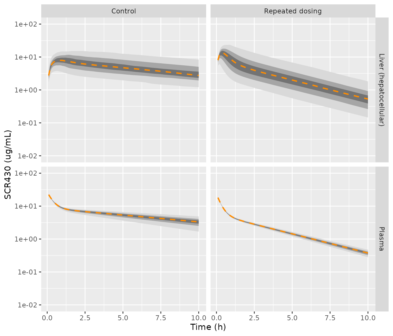

Replicates Figure 8 of Kim 2022: 5th-95th, 20th-80th and 35th-65th percentile bands and the median of simulated plasma (top) and hepatocellular (bottom) SCR430 after 3 mg/kg IV.

Read off Figure 8, the paper’s median curves run from about 25 to 4 ug/mL (control plasma) and 22 to 0.45 ug/mL (repeated-dosing plasma) between the first sample and 10 h. The hepatocellular medians peak near 7 ug/mL at 1 h (control) and near 8 to 9 ug/mL within the first half hour (repeated dosing), ending near 4 and 0.45 ug/mL at 10 h. The simulated percentiles at selected times are below. The early repeated-dosing hepatocellular median (about 13 ug/mL at 0.5 h) runs higher than the figure’s; the plasma medians and the 10 h values agree within the reading precision of the log-scale figure.

mc_q |>
  filter(time %in% c(0.5, 1, 2, 10)) |>
  select(group, output, time, q05, q50, q95) |>
  arrange(output, group, time) |>
  knitr::kable(digits = 2)

group	output	time	q05	q50	q95
Control	Liver (hepatocellular)	0.5	3.70	7.44	12.38
Control	Liver (hepatocellular)	1.0	3.51	7.89	14.78
Control	Liver (hepatocellular)	2.0	2.68	6.58	15.23
Control	Liver (hepatocellular)	10.0	1.21	2.76	8.38
Repeated dosing	Liver (hepatocellular)	0.5	3.73	12.82	22.89
Repeated dosing	Liver (hepatocellular)	1.0	2.07	8.20	22.41
Repeated dosing	Liver (hepatocellular)	2.0	1.35	4.67	15.70
Repeated dosing	Liver (hepatocellular)	10.0	0.15	0.53	1.82
Control	Plasma	0.5	11.44	12.49	13.12
Control	Plasma	1.0	7.66	8.83	9.58
Control	Plasma	2.0	5.83	7.18	8.09
Control	Plasma	10.0	1.68	3.31	4.87
Repeated dosing	Plasma	0.5	7.68	8.05	8.39
Repeated dosing	Plasma	1.0	4.50	4.83	5.13
Repeated dosing	Plasma	2.0	2.95	3.25	3.52
Repeated dosing	Plasma	10.0	0.28	0.38	0.47

med10 <- mc_q |> filter(time == 10)
pl_ctl <- med10$q50[med10$group == "Control" & med10$output == "Plasma"]
pl_rep <- med10$q50[med10$group == "Repeated dosing" & med10$output == "Plasma"]
stopifnot(
  # Median plasma at 10 h within a factor of 1.5 of the Figure 8 median
  # (read off a log axis: about 4 and 0.45 ug/mL).
  pl_ctl > 4 / 1.5, pl_ctl < 4 * 1.5,
  pl_rep > 0.45 / 1.5, pl_rep < 0.45 * 1.5,
  # The induction effect: an order of magnitude between the groups at 10 h.
  pl_ctl / pl_rep > 5
)

PKNCA validation against Table 1

The paper’s non-compartmental analysis (PKSolver) used plasma sampled to 10 h. The schedule below approximates the Figure 2a sampling times; AUC0-inf is extrapolated from the terminal phase, as in the paper.

nca_times <- c(0, 0.083, 0.25, 0.5, 1, 2, 3, 4, 7, 10)
make_nca_events <- function(group, n, id_offset = 0L) {
  rxode2::et(amt = 3, cmt = "central") |>
    rxode2::et(nca_times, cmt = "central") |>
    as.data.frame() |>
    # Two `~` endpoints (Cc, Cliver): observation rows carry dvid = 1; the
    # forward solve still returns both concentration columns.
    mutate(dvid = ifelse(evid == 0, 1L, NA_integer_)) |>
    tidyr::crossing(id = id_offset + seq_len(n)) |>
    select(-any_of("ID")) |>
    relocate(id) |>
    arrange(id, time, desc(evid)) |>
    mutate(group = group)
}
sim_nca <- bind_rows(
  as.data.frame(rxode2::rxSolve(mod_ctl, make_nca_events("Control", n_mc), keep = "group")),
  as.data.frame(rxode2::rxSolve(mod_rep, make_nca_events("Repeated dosing", n_mc, n_mc), keep = "group"))
) |>
  filter(!is.na(Cc)) |>
  select(id, time, Cc, group) |>
  distinct(id, group, time, .keep_all = TRUE) |>
  arrange(id, time)

dose_df <- sim_nca |> distinct(id, group) |> mutate(time = 0, dose = 3)

conc_obj <- PKNCAconc(sim_nca, Cc ~ time | group + id, concu = "ug/mL", timeu = "h")
dose_obj <- PKNCAdose(dose_df, dose ~ time | group + id, route = "intravascular", doseu = "mg/kg")
intervals <- data.frame(
  start = 0, end = Inf,
  auclast = FALSE, aucinf.obs = TRUE, cl.obs = TRUE, vss.obs = TRUE, half.life = TRUE
)
nca <- pk.nca(PKNCAdata(conc_obj, dose_obj, intervals = intervals))
nca_res <- as.data.frame(nca$result)

Table 1 reports AUC in ug/mLmin (6333 and 1420); dividing by 60 gives 105.6 and 23.7 ugh/mL.

ref <- data.frame(
  group = c("Control", "Repeated dosing"),
  aucinf.obs = c(6333, 1420) / 60, # Table 1, ug/mL*min -> ug*h/mL
  cl.obs = c(30.02, 137.9) / 1000, # Table 1, mL/h/kg -> L/h/kg
  vss.obs = c(286.4, 378.4) / 1000 # Table 1, mL/kg -> L/kg
)
cmp <- ncaComparisonTable(
  simulated = nca_res,
  reference = ref,
  by = "group",
  params = c("aucinf.obs", "cl.obs", "vss.obs"),
  units = c(aucinf.obs = "ug*h/mL", cl.obs = "L/h/kg", vss.obs = "L/kg")
)
knitr::kable(cmp)

NCA parameter	group	Reference	Simulated	% diff
AUC0-∞ (obs) (ug*h/mL)	Control	106	96.5	-8.5%
AUC0-∞ (obs) (ug*h/mL)	Repeated dosing	23.7	26.5	+12.1%
CL/F (L/h/kg)	Control	0.03	0.0311	+3.5%
CL/F (L/h/kg)	Repeated dosing	0.138	0.113	-18.0%
Vss/F (L/kg)	Control	0.286	0.298	+4.0%
Vss/F (L/kg)	Repeated dosing	0.378	0.332	-12.3%

nca_med <- nca_res |>
  filter(PPTESTCD %in% c("aucinf.obs", "cl.obs")) |>
  group_by(group, PPTESTCD) |>
  summarise(med = median(PPORRES, na.rm = TRUE), .groups = "drop")
auc_ratio <- nca_med$med[nca_med$group == "Control" & nca_med$PPTESTCD == "aucinf.obs"] /
  nca_med$med[nca_med$group == "Repeated dosing" & nca_med$PPTESTCD == "aucinf.obs"]
auc_ratio
#> [1] 3.639361
stopifnot(
  # Observed control-to-repeated AUC ratio is 4.5 (Table 1); the model's
  # median ratio must land in the same range.
  auc_ratio > 3, auc_ratio < 6,
  # Median clearance within 30% of the Table 1 group means.
  abs(nca_med$med[nca_med$group == "Control" & nca_med$PPTESTCD == "cl.obs"] / 0.03002 - 1) < 0.3,
  abs(nca_med$med[nca_med$group == "Repeated dosing" & nca_med$PPTESTCD == "cl.obs"] / 0.1379 - 1) < 0.3
)

The simulated medians land within about 20% of the observed group means for AUC and clearance in both groups, and within about 12% for Vss. Vss was not a fitting target; only the plasma profile was fitted.

Assumptions and deviations

• Two files, one structure. The paper runs one mPBPK structure with two sets of hepatocyte-derived inputs (Table 3). The volume and exchange rate constants are “Equal to Control”. The two sets are packaged as two files so that each carries its own variability magnitudes. A covariate to switch between them is not needed.
• Systemic and single-adjustment equations. Appendix A.2 prints only the liver equations. The systemic compartment’s mass balance is read from the Figure 7 schematic: hepatic blood flow leaves into Inlet 1 and returns from Inlet 5, and kin / kout act first-order on the systemic and single-adjustment amounts. Because kin / kout act on amounts, the single-adjustment compartment needs no volume. That is consistent with Table 3 listing none, although Section 3.7 says that compartment’s volume was fitted.
• Blood vs plasma. Eq. A1 multiplies the systemic concentration by the hepatic BLOOD flow, and uptake acts on fu,b * Che. The systemic compartment therefore holds blood concentration, and plasma is blood / Rb, using each group’s Table 1 Rb. With this reading the model’s steady-state volume is about 0.30 L/kg (control; see the PKNCA table), against the observed Vdss of 0.29 L/kg. Treating the systemic compartment as plasma would give about 0.1 L/kg.
• Liver output. Cliver is the mean hepatocellular concentration. The paper measured liver concentrations after correcting for blood left in the tissue (Eq. 1), and the hepatocellular mean reproduces the Figure 8c/8d median curves. Averaging the extracellular blood units in as well gives values about twice as high.
• The 1.6-fold scaling factor is applied to both PSinf,act and PSdiff on top of the Table 3 values, per Section 3.7. The Table 3 values sum to the unscaled Method 2 PSinf (see the IVIVE check above). Without the factor, the repeated-dosing clearance would be about 75 mL/h/kg against the observed 137.9.
• Text vs Table 3 for PSdiff. Section 3.7 states PSdiff as 0.8 and 0.6 L/h/kg. Those are the standard deviations of PSinf,act in Table 3. The Table 3 PSdiff means (0.3 and 0.86 L/h/kg) are used because they reproduce the Method 2 PSinf.
• CLint,met (control). Table 3 lists 9.8 L/h/kg, while Table 2’s 160.4 mL/min/kg converts to 9.6 L/h/kg. The Table 3 value is the mPBPK input and is used.
• Lognormal centring. The paper’s Monte Carlo distributions are parameterised by their arithmetic mean (Eqs. 17 to 19). The typical values are the medians of those distributions, so the etas reproduce the paper’s Monte Carlo draw exactly. A typical-value (no-eta) solve therefore uses the median, below the Table 3 mean by up to 28 percent (the largest gap is fu,hepa in the repeated-dosing group; PSinf,act and CLint,met there differ by well under 1 percent). The eta variances are the Eq. 18 values and are held constant, because they come from in vitro assay variability and were not estimated.
• No residual error is reported; both proportional residual SDs are fixed at zero.
• Vehicle group and intraperitoneal data (Table 1, Figure 2b) were not modelled by the paper and are not part of either file.