Teicoplanin in children (Zhang 2020)
Source:vignettes/articles/Zhang_2020_teicoplanin.Rmd
Zhang_2020_teicoplanin.RmdModel and source
ui <- rxode2::rxode(readModelDb("Zhang_2020_teicoplanin"))
#> ℹ parameter labels from comments will be replaced by 'label()'- Citation: Zhang T, Sun D, Shu Z, Duan Z, Liu Y, Du Q, Zhang Y, Dong Y, Wang T, Hu S, Cheng H, Dong Y. Population Pharmacokinetics and Model-Based Dosing Optimization of Teicoplanin in Pediatric Patients. Front Pharmacol. 2020;11:594562. doi:10.3389/fphar.2020.594562
- Description: One-compartment IV population PK model for teicoplanin in 159 hospitalised Chinese children aged 1 month to 14 years (Zhang 2020). Clearance carries a linear body-weight term and an exponential serum-creatinine term, CL = 0.0694 * (1 + 2.82 * WT/16.71) * 0.882^(SCr/29.075), and the volume of distribution an exponential body-weight term, V = 1.39 * 1.75^(WT/16.71); 16.71 kg and 29.075 umol/L are the cohort means. For a child at those means CL = 0.234 L/h (0.014 L/h/kg) and V = 2.43 L (0.15 L/kg). Interindividual variability is exponential on CL (65.9% CV) and V (61.0% CV), and residual variability is 7.0% proportional.
- Article (DOI): https://doi.org/10.3389/fphar.2020.594562
Zhang 2020 fitted a one-compartment model with first-order elimination (NONMEM 7.2, ADVAN1 TRANS2, FOCE-I) to 236 sparse teicoplanin concentrations, mostly steady-state troughs, from 159 hospitalised children in two hospitals in Xi’an, China. Body weight and serum creatinine were retained on clearance and body weight on the volume of distribution. The paper then used Monte Carlo simulation to recommend loading and maintenance doses by weight and creatinine band (Table 3).
mod <- readModelDb("Zhang_2020_teicoplanin")
mod
#> function() {
#>   description <- "One-compartment IV population PK model for teicoplanin in 159 hospitalised Chinese children aged 1 month to 14 years (Zhang 2020). Clearance carries a linear body-weight term and an exponential serum-creatinine term, CL = 0.0694 * (1 + 2.82 * WT/16.71) * 0.882^(SCr/29.075), and the volume of distribution an exponential body-weight term, V = 1.39 * 1.75^(WT/16.71); 16.71 kg and 29.075 umol/L are the cohort means. For a child at those means CL = 0.234 L/h (0.014 L/h/kg) and V = 2.43 L (0.15 L/kg). Interindividual variability is exponential on CL (65.9% CV) and V (61.0% CV), and residual variability is 7.0% proportional."
#>   reference <- "Zhang T, Sun D, Shu Z, Duan Z, Liu Y, Du Q, Zhang Y, Dong Y, Wang T, Hu S, Cheng H, Dong Y. Population Pharmacokinetics and Model-Based Dosing Optimization of Teicoplanin in Pediatric Patients. Front Pharmacol. 2020;11:594562. doi:10.3389/fphar.2020.594562"
#>   vignette <- "Zhang_2020_teicoplanin"
#>   units <- list(time = "h", dosing = "mg", concentration = "mg/L")
#>
#>   # What each ODE state holds, in what amount units, in what biological matrix.
#>   # Zhang 2020 Methods: teicoplanin in serum by a validated HPLC method
#>   # (calibration 2.5-100 mg/L, LLOQ 2.5 mg/L).
#>   compartmentData <- list(
#>     central = list(analyte = "teicoplanin", units = "mg", specimen = "serum", verified = TRUE)
#>   )
#>
#>   covariateData <- list(
#>     WT = list(
#>       description = "Body weight",
#>       units = "kg",
#>       type = "continuous",
#>       notes = "Enters CL linearly as (1 + 2.82 * WT/16.71) and V exponentially as 1.75^(WT/16.71) (Zhang 2020 Results, final-model equations). 16.71 kg is the model-building cohort mean (Table 1: 16.7 +/- 10.1 kg, median 14.8, range 2.9-69.0). Both terms are anchored at WT = 0 rather than at the cohort mean, so the typical values lcl and lvc are NOT the values for a typical child; see ini().",
#>       source_name = "WT"
#>     ),
#>     CREAT = list(
#>       description = "Serum creatinine",
#>       units = "umol/L",
#>       type = "continuous",
#>       notes = "Enters CL exponentially as 0.882^(SCr/29.075) (Zhang 2020 Results, final-model equation). 29.075 umol/L is the model-building cohort mean (Table 1: 29.1 +/- 17.3 umol/L, median 26.0, range 10.0-139.0). Higher creatinine lowers clearance. If no creatinine reading fell within +/- 48 h of dosing the closest available reading was imputed (12 of 236 samples, 5.1%).",
#>       source_name = "SCr"
#>     )
#>   )
#>
#>   # Screened in the stepwise covariate search (Zhang 2020 Methods, Supplementary
#>   # Table S3) but NOT retained in the final model. Documentation only -- none of
#>   # these appears in model().
#>   covariatesDataExcluded <- list(
#>     AGE = list(
#>       description = "Subject age",
#>       units = "years",
#>       type = "continuous",
#>       notes = "Table 1: 4.1 +/- 3.4 years (median 3.7, range 0.2-14.0). Age on V entered the full model in forward selection (Supplementary Table S3 model 3, dOFV -28.6) but was removed in backward elimination (model 7, dOFV +0.014)."
#>     ),
#>     SEXF = list(
#>       description = "Biological sex indicator, 1 = female, 0 = male",
#>       units = "(binary)",
#>       type = "binary",
#>       notes = "Table 1: 72 of 159 (45.3%) female. Screened but not retained."
#>     ),
#>     CRCL = list(
#>       description = "Creatinine clearance (Cockcroft-Gault)",
#>       units = "mL/min",
#>       type = "continuous",
#>       notes = "Table 1: 87.8 +/- 47.2 mL/min. Computed with the Cockcroft-Gault formula because height was unavailable for most children; screened but not retained. The Discussion attributes this to Cockcroft-Gault overestimating renal function in small children."
#>     ),
#>     BUN = list(
#>       description = "Blood urea nitrogen",
#>       units = "(not reported)",
#>       type = "continuous",
#>       notes = "Screened (Methods) but not retained; no summary statistics reported."
#>     ),
#>     TPRO = list(
#>       description = "Serum total protein",
#>       units = "(not reported)",
#>       type = "continuous",
#>       notes = "Screened (Methods) but not retained; no summary statistics reported."
#>     ),
#>     ALB = list(
#>       description = "Serum albumin",
#>       units = "(not reported)",
#>       type = "continuous",
#>       notes = "Screened (Methods) but not retained; no summary statistics reported."
#>     )
#>   )
#>
#>   population <- list(
#>     species = "human",
#>     n_subjects = 159L,
#>     n_studies = 1L,
#>     n_concentrations = 236L,
#>     age_range = "Mean 4.1 +/- 3.4 years, median 3.7, range 0.2-14.0 years; 51 (32.1%) under 2 years, 98 (61.6%) 2-10 years, 10 (6.3%) 10 years and over (Zhang 2020 Table 1). Eligibility was 1 month to 18 years.",
#>     weight_range = "Mean 16.7 +/- 10.1 kg, median 14.8, range 2.9-69.0 kg (Table 1)",
#>     sex_female_pct = 45.3,
#>     race_ethnicity = "Chinese (two hospitals in Xi'an, China); described by the authors as an Asian paediatric population",
#>     disease_state = "Hospitalised children receiving teicoplanin for proven or suspected MRSA infection. Indications (not mutually exclusive): respiratory tract infection 97.5%, sepsis 24.5%, bacteraemia 12.6%, bone and joint infection 6.9%. Comorbidities: malignant haematological disease 57.2%, congenital heart disease 15.1%, myocardial injury 13.8%. 30.2% ventilated, 25.2% admitted to intensive care (Table 1).",
#>     dose_range = "Three loading doses of 10 mg/kg every 12 h, then 6-10 mg/kg/day (label regimen). Received: loading dose 9.8 +/- 1.4 mg/kg (range 5.2-16.0); daily maintenance dose 9.5 +/- 1.2 mg/kg (range 5.2-12.9) (Table 1). Infusion duration not reported.",
#>     regions = "China (First Affiliated Hospital and Affiliated Children Hospital of Xi'an Jiaotong University)",
#>     renal_function = "Serum creatinine 29.1 +/- 17.3 umol/L (median 26.0, range 10.0-139.0); Cockcroft-Gault creatinine clearance 87.8 +/- 47.2 mL/min (Table 1).",
#>     co_medication = "Other antibacterials: ceftriaxone 42.8%, meropenem 34.0%, imipenem-cilastatin 45.3%, cefoperazone-sulbactam 19.5%; loop diuretic 42.8% (Table 1). Nephrotoxic co-medication was screened but not retained.",
#>     notes = "Retrospective study, March 2017 to November 2019. Sparse data: 236 concentrations, 1.5 per child, 212 (89.8%) of them TDM troughs drawn within 30 min before a dose at steady state; six below the 2.5 mg/L LLOQ were set to 2.5 mg/L. NONMEM 7.2, ADVAN1 TRANS2, FOCE-I. Final-model OFV 971.014. Shrinkage 26.9% (CL), 19.8% (V), 24.4% (residual). The model was externally evaluated on a separate cohort of 66 children (89 concentrations) from the same hospitals; that cohort is not part of the fit."
#>   )
#>
#>   ini({
#>     # Structural parameters from Zhang 2020 Table 2 ('Final model' column),
#>     # confirmed by the final-model equations printed in the Results:
#>     #   CL (L/h) = 0.0694 x (1 + theta1 x WT/16.71) x theta2^(SCr/29.075) x e^eta1
#>     #   Vd (L)   = 1.39 x theta3^(WT/16.71) x e^eta2
#>     # Both are anchored at WT = 0 (and SCr = 0), so these two values are not the
#>     # values of any real child. The abstract's 'clearance ... 0.694 L/h' drops a
#>     # zero: Table 2 and the equation both give 0.0694, and only 0.0694
#>     # reproduces the abstract's own '0.784 L/h/70 kg' (see e_creat_cl below).
#>     lcl <- log(0.0694); label("Clearance at WT = 0 and SCr = 0 (L/h)")                 # Table 2: CL = 0.0694 L/h (RSE 11.3%; bootstrap mean 0.0718, 95% CI 0.0453-0.0983)
#>     lvc <- log(1.39); label("Volume of distribution at WT = 0 (L)")                  # Table 2: Vd = 1.39 L (RSE 11.0%; bootstrap mean 1.77, 95% CI 1.34-2.20)
#>
#>     # Covariate effects. The printed equation image shows theta2 and theta3 as
#>     # BASES raised to the covariate ratio (theta^(cov/ref)), not as power
#>     # exponents on the ratio ((cov/ref)^theta). Three of the paper's own derived
#>     # numbers reproduce only under the base reading:
#>     #   CL at WT 16.71, SCr 29.075 = 0.0694 * 3.82 * 0.882 = 0.2338 L/h
#>     #     = 0.0140 L/h/kg (Discussion: '0.014 L/h/kg'); the power reading gives 0.0159.
#>     #   CL at WT 70, SCr 29.075 = 0.0694 * 12.813 * 0.882 = 0.784 L/h
#>     #     (Abstract: '0.784 L/h/70 kg'); the power reading gives 0.889.
#>     #   Vd at WT 16.71 = 1.39 * 1.75 = 2.43 L = 0.146 L/kg
#>     #     (Discussion: 'Vd in this study (0.15 L/kg)'); the power reading gives 0.083.
#>     e_wt_cl <- 2.82; label("Linear slope of CL on WT/16.71 (unitless)")               # Table 2: theta_wt on CL = 2.82 (RSE 20.6%; bootstrap mean 3.62, 95% CI 1.21-6.03)
#>     e_creat_cl <- 0.882; label("Base of the exponential SCr effect on CL, theta^(SCr/29.075) (unitless)") # Table 2: theta_SCr on CL = 0.882 (RSE 5.0%; bootstrap mean 0.794, 95% CI 0.688-0.9)
#>     e_wt_vc <- 1.75; label("Base of the exponential WT effect on Vd, theta^(WT/16.71) (unitless)")      # Table 2: theta_wt on Vd = 1.75 (RSE 6.3%; bootstrap mean 1.76, 95% CI 1.29-2.23)
#>
#>     # IIV: exponential model (Methods), reported in Table 2 as CV%. Converted with
#>     # omega^2 = log(1 + CV^2); the paper gives no CI, equation exponent or
#>     # variance column that would settle the convention otherwise.
#>     etalcl ~ 0.3607 # Table 2: CV-CL = 65.9% (RSE 17.6%); log(1 + 0.659^2) = 0.3607
#>     etalvc ~ 0.3163 # Table 2: CV-Vd = 61.0% (RSE 42.5%); log(1 + 0.610^2) = 0.3163
#>
#>     # Residual error: Table 2 reports 'Residual variability (%)', 'CV-sigma' =
#>     # 7.0%. The Results say an additive model was selected, and a CV% label on an
#>     # additive error means additive on the log-transformed scale, i.e.
#>     # proportional on the linear scale. A 7.0 mg/L additive SD is ruled out by
#>     # Figure 3: its lower 5th-percentile band stays at 0-5 mg/L, whereas a
#>     # 7 mg/L additive SD at a median of ~10 mg/L would put it well below zero.
#>     propSd <- 0.07; label("Proportional residual error (fraction)")                    # Table 2: CV-sigma = 7.0% (RSE 21.9%; bootstrap mean 8.5, 95% CI 5.1-11.9)
#>   })
#>   model({
#>     # Individual PK parameters (Zhang 2020 Results, final-model equations).
#>     # 16.71 kg and 29.075 umol/L are the model-building cohort means (Table 1).
#>     cl <- exp(lcl + etalcl) * (1 + e_wt_cl * WT / 16.71) * e_creat_cl^(CREAT / 29.075)
#>     vc <- exp(lvc + etalvc) * e_wt_vc^(WT / 16.71)
#>
#>     kel <- cl / vc
#>
#>     # One-compartment model with first-order elimination (ADVAN1 TRANS2).
#>     # Doses (mg) enter central as IV infusions; the infusion duration was not
#>     # reported and is set in the event table.
#>     d/dt(central) <- -kel * central
#>
#>     Cc <- central / vc
#>     Cc ~ prop(propSd)
#>   })
#> }
#> <environment: 0x55aa125ada10>
Population
tibble::tribble(
  ~Characteristic,                         ~Value,
  "Children (concentrations)",             "159 (236; 1.5 per child; 89.8% TDM troughs)",
  "Male / female",                         "87 (54.7%) / 72 (45.3%)",
  "Age (years)",                           "4.1 +/- 3.4 (median 3.7, range 0.2-14.0)",
  "Age < 2 / 2-10 / >= 10 years",          "51 (32.1%) / 98 (61.6%) / 10 (6.3%)",
  "Weight (kg)",                           "16.7 +/- 10.1 (median 14.8, range 2.9-69.0)",
  "Serum creatinine (umol/L)",             "29.1 +/- 17.3 (median 26.0, range 10.0-139.0)",
  "Creatinine clearance, C-G (mL/min)",    "87.8 +/- 47.2 (median 89.6)",
  "Malignant haematological disease",      "91 (57.2%)",
  "Intensive care / ventilated",           "40 (25.2%) / 48 (30.2%)",
  "Loading dose (mg/kg)",                  "9.8 +/- 1.4 (median 10.0)",
  "Daily maintenance dose (mg/kg)",        "9.5 +/- 1.2 (median 10.0)",
  "Observed concentration (mg/L)",         "8.6 +/- 12.1 (median 10.3, range 2.5-82.3)"
) |>
knitr::kable(caption = "Zhang 2020 Table 1, model-building cohort; mean +/- SD (median, range).")| Characteristic | Value |
|---|---|
| Children (concentrations) | 159 (236; 1.5 per child; 89.8% TDM troughs) |
| Male / female | 87 (54.7%) / 72 (45.3%) |
| Age (years) | 4.1 +/- 3.4 (median 3.7, range 0.2-14.0) |
| Age < 2 / 2-10 / >= 10 years | 51 (32.1%) / 98 (61.6%) / 10 (6.3%) |
| Weight (kg) | 16.7 +/- 10.1 (median 14.8, range 2.9-69.0) |
| Serum creatinine (umol/L) | 29.1 +/- 17.3 (median 26.0, range 10.0-139.0) |
| Creatinine clearance, C-G (mL/min) | 87.8 +/- 47.2 (median 89.6) |
| Malignant haematological disease | 91 (57.2%) |
| Intensive care / ventilated | 40 (25.2%) / 48 (30.2%) |
| Loading dose (mg/kg) | 9.8 +/- 1.4 (median 10.0) |
| Daily maintenance dose (mg/kg) | 9.5 +/- 1.2 (median 10.0) |
| Observed concentration (mg/L) | 8.6 +/- 12.1 (median 10.3, range 2.5-82.3) |
The label regimen is three loading doses of 10 mg/kg every 12 h followed by 6-10 mg/kg once daily. The infusion duration is not reported.
Source trace
tibble::tribble(
  ~Quantity,                          ~`Model file`,  ~Value,          ~`Source location`,
  "CL at WT = 0, SCr = 0",            "lcl",          "0.0694 L/h",    "Table 2 (RSE 11.3%); Results CL equation",
  "Vd at WT = 0",                     "lvc",          "1.39 L",        "Table 2 (RSE 11.0%); Results Vd equation",
  "Linear WT slope on CL",            "e_wt_cl",      "2.82",          "Table 2 theta_wt on CL (RSE 20.6%)",
  "Base of SCr term on CL",           "e_creat_cl",   "0.882",         "Table 2 theta_SCr on CL (RSE 5.0%)",
  "Base of WT term on Vd",            "e_wt_vc",      "1.75",          "Table 2 theta_wt on Vd (RSE 6.3%)",
  "IIV on CL",                        "etalcl",       "0.3607",        "Table 2 CV-CL 65.9%; log(1 + CV^2)",
  "IIV on Vd",                        "etalvc",       "0.3163",        "Table 2 CV-Vd 61.0%; log(1 + CV^2)",
  "Residual error",                   "propSd",       "0.07",          "Table 2 CV-sigma 7.0%",
  "WT centring value",                "16.71 kg",     "cohort mean",   "Results equations; Table 1 mean 16.7",
  "SCr centring value",               "29.075 umol/L","cohort mean",   "Results equations; Table 1 mean 29.1",
  "Structure",                        "d/dt(central)","1-cmt, IV",     "Methods (ADVAN1 TRANS2)"
) |>
knitr::kable(caption = "Source location of every ini() value and structural choice.")| Quantity | Model file | Value | Source location |
|---|---|---|---|
| CL at WT = 0, SCr = 0 | lcl | 0.0694 L/h | Table 2 (RSE 11.3%); Results CL equation |
| Vd at WT = 0 | lvc | 1.39 L | Table 2 (RSE 11.0%); Results Vd equation |
| Linear WT slope on CL | e_wt_cl | 2.82 | Table 2 theta_wt on CL (RSE 20.6%) |
| Base of SCr term on CL | e_creat_cl | 0.882 | Table 2 theta_SCr on CL (RSE 5.0%) |
| Base of WT term on Vd | e_wt_vc | 1.75 | Table 2 theta_wt on Vd (RSE 6.3%) |
| IIV on CL | etalcl | 0.3607 | Table 2 CV-CL 65.9%; log(1 + CV^2) |
| IIV on Vd | etalvc | 0.3163 | Table 2 CV-Vd 61.0%; log(1 + CV^2) |
| Residual error | propSd | 0.07 | Table 2 CV-sigma 7.0% |
| WT centring value | 16.71 kg | cohort mean | Results equations; Table 1 mean 16.7 |
| SCr centring value | 29.075 umol/L | cohort mean | Results equations; Table 1 mean 29.1 |
| Structure | d/dt(central) | 1-cmt, IV | Methods (ADVAN1 TRANS2) |
The final-model equations printed in the Results are
CL (L/h) = 0.0694 x (1 + theta1 x WT/16.71) x theta2^(SCr/29.075) x e^eta1
Vd (L)   = 1.39 x theta3^(WT/16.71) x e^eta2
with theta1 = 2.82, theta2 = 0.882 and theta3 = 1.75 (Table 2). theta2 and theta3 are bases raised to the covariate ratio, not exponents on it. The next section shows that the paper’s own derived numbers reproduce only under that reading.
Typical-value identities
The paper quotes three derived quantities: a typical clearance of 0.014 L/h/kg and a volume of 0.15 L/kg (Discussion), and a clearance of 0.784 L/h for a 70 kg child (Abstract). The table below computes each one from the packaged model under the printed form (theta as a base), and under the alternative reading (theta as a power exponent on the covariate ratio).
# The typical-value solves switch the random effects off. rxode2 then notes a
# multi-subject simulation without 'omega', which is expected here.
solve_fixed <- function(...) {
  withCallingHandlers(
    rxSolve(...),
    warning = function(w) {
      if (grepl("without .*'omega'", conditionMessage(w))) invokeRestart("muffleWarning")
    }
  )
}
mod_typ <- zeroRe(mod)
#> ℹ parameter labels from comments will be replaced by 'label()'
ref <- tibble::tibble(
  id    = 1:2,
  WT    = c(16.71, 70),
  CREAT = c(29.075, 29.075)
)
ev_ref <- et(amt = 100, time = 0, dur = 0.5, cmt = "central") |>
  et(time = 1, cmt = "central") |>
  et(id = 1:2)
typ <- solve_fixed(mod_typ, as.data.frame(ev_ref) |> left_join(ref, by = "id"),
                   returnType = "data.frame", addDosing = FALSE) |>
  distinct(id, cl, vc) |>
  left_join(ref, by = "id")
#> ℹ omega/sigma items treated as zero: 'etalcl', 'etalvc'

power_form <- function(wt, scr) {
  c(cl = 0.0694 * (1 + 2.82 * wt / 16.71) * (scr / 29.075)^0.882,
    vc = 1.39 * (wt / 16.71)^1.75)
}

tab_id <- tibble::tibble(
  Quantity  = c("CL/WT at the cohort means (L/h/kg)", "Vd/WT at the cohort means (L/kg)",
                "CL at 70 kg (L/h)"),
  Paper     = c(0.014, 0.15, 0.784),
  `Packaged model` = c(typ$cl[1] / 16.71, typ$vc[1] / 16.71, typ$cl[2]),
  `Power-exponent reading` = c(power_form(16.71, 29.075)[["cl"]] / 16.71,
                               power_form(16.71, 29.075)[["vc"]] / 16.71,
                               power_form(70, 29.075)[["cl"]])
)
knitr::kable(tab_id, digits = 4, caption = "Derived quantities quoted in Zhang 2020.")| Quantity | Paper | Packaged model | Power-exponent reading |
|---|---|---|---|
| CL/WT at the cohort means (L/h/kg) | 0.014 | 0.0140 | 0.0159 |
| Vd/WT at the cohort means (L/kg) | 0.150 | 0.1456 | 0.0832 |
| CL at 70 kg (L/h) | 0.784 | 0.7843 | 0.8892 |
# Deterministic: all three reproduce to the paper's printed precision under the
# base reading (0.01399, 0.1456, 0.7843), and none does under the power reading
# (0.0159, 0.083, 0.889).
stopifnot(
  abs(typ$cl[1] / 16.71 - 0.014) < 0.0005,
  abs(typ$vc[1] / 16.71 - 0.15) < 0.005,
  abs(typ$cl[2] - 0.784) < 0.0005
)
For the typical child at the cohort means (16.71 kg, 29.075 umol/L) the model gives CL = 0.234 L/h and Vd = 2.43 L, an elimination half-life of about 7 h. That is much shorter than the 30-180 h usually quoted for teicoplanin in adults, and the Vd of 0.15 L/kg is small. It is what the model says: the paper fitted a single compartment to sparse, mostly trough data, which cannot separate a distribution phase from terminal elimination. The paper itself compares its 0.15 L/kg with the 0.2 L/kg of Ramos-Martin 2014.
Covariate directions
Table 3 recommends larger mg/kg doses for lighter children and for children with lower creatinine. So at a fixed mg/kg dose the trough must rise with body weight and with creatinine. The typical-value check below uses the standard 10 mg/kg loading regimen and reads the trough at 48 h.
grid <- tidyr::expand_grid(WT = c(5, 15, 25, 40), CREAT = c(30, 60)) |>
  mutate(id = row_number())

make_events <- function(cohort, mgkg, dose_times, obs_times, dur = 0.5) {
  dose <- tidyr::expand_grid(id = cohort$id, time = dose_times) |>
    left_join(cohort, by = "id") |>
    mutate(amt = mgkg * WT, dur = dur, evid = 1L, cmt = "central")
  obs <- tidyr::expand_grid(id = cohort$id, time = obs_times) |>
    left_join(cohort, by = "id") |>
    mutate(amt = 0, dur = 0, evid = 0L, cmt = "central")
  bind_rows(dose, obs) |> arrange(id, time, desc(evid))
}

dir_sim <- solve_fixed(mod_typ, make_events(grid, 10, c(0, 12, 24), 48),
                       returnType = "data.frame", addDosing = FALSE)
#> ℹ omega/sigma items treated as zero: 'etalcl', 'etalvc'

dir_sim |>
  select(WT, CREAT, Cc) |>
  tidyr::pivot_wider(names_from = CREAT, values_from = Cc, names_prefix = "SCr ") |>
  knitr::kable(digits = 2,
caption = "Typical trough at 48 h (mg/L) after 10 mg/kg q12h x 3, by weight and creatinine.")| WT | SCr 30 | SCr 60 |
|---|---|---|
| 5 | 9.79 | 12.58 |
| 15 | 10.08 | 13.96 |
| 25 | 10.34 | 14.53 |
| 40 | 13.29 | 18.16 |
# Deterministic typical-value solves.
cmin_by <- function(wt, scr) dir_sim$Cc[dir_sim$WT == wt & dir_sim$CREAT == scr]
stopifnot(
  nrow(dir_sim) == nrow(grid),
  all(diff(dir_sim$Cc[dir_sim$CREAT == 30]) > 0),
  all(diff(dir_sim$Cc[dir_sim$CREAT == 60]) > 0),
  all(vapply(c(5, 15, 25, 40), function(w) cmin_by(w, 60) > cmin_by(w, 30), logical(1)))
)
Both directions match the paper.
Virtual cohort
Zhang 2020 simulated 5,000 virtual children. This vignette uses 200 per regimen. Random draws from 200 subjects are too noisy here: the cohort mean trough moved by about 35% between seeds while this vignette was being written. So the cohort is a deterministic low-discrepancy (Halton) lattice over the four random inputs: body weight, serum creatinine and the two etas. It uses the same 200 children for every regimen. The lattice uses no random number generator, so every number below is the same on every machine.
- Body weight: log-normal, median 14.8 kg, log-scale SD 0.49 (which reproduces Table 1’s mean of 16.7 kg), truncated to the observed 2.9-69.0 kg.
- Serum creatinine: log-normal, median 26.0 umol/L, log-scale SD 0.475 (reproducing the mean of 29.1), truncated to 10-139 umol/L. It is correlated with weight at 0.5 on the log scale. The paper gives no correlation, but in Supplementary Table S2 the older, heavier Hospital 1 children have the higher creatinine. Changing the correlation between 0 and 0.7 moves the mean trough by less than 1%.
- Etas: normal with the model’s variances.
Truncation is applied in quantile space, which is equivalent to rejecting and redrawing. It never clamps.
halton <- function(n, base) {
  vapply(seq_len(n), function(i) {
    f <- 1
    r <- 0
    while (i > 0) {
      f <- f / base
      r <- r + f * (i %% base)
      i <- i %/% base
    }
    r
  }, numeric(1))
}

omega <- ui$omega
build_lattice <- function(n, rho = 0.5) {
  u <- cbind(halton(n, 2), halton(n, 3), halton(n, 5), halton(n, 7))
  zb <- function(x, med, s) (log(x) - log(med)) / s
  pl <- pnorm(zb(2.9, 14.8, 0.49))
  pu <- pnorm(zb(69, 14.8, 0.49))
  zw <- qnorm(pl + u[, 1] * (pu - pl))
  mu <- rho * zw
  s <- sqrt(1 - rho^2)
  pl2 <- pnorm((zb(10, 26, 0.475) - mu) / s)
  pu2 <- pnorm((zb(139, 26, 0.475) - mu) / s)
  zs <- mu + s * qnorm(pl2 + u[, 2] * (pu2 - pl2))
  tibble::tibble(
    id     = seq_len(n),
    WT     = 14.8 * exp(0.49 * zw),
    CREAT  = 26 * exp(0.475 * zs),
    etalcl = sqrt(omega["etalcl", "etalcl"]) * qnorm(u[, 3]),
    etalvc = sqrt(omega["etalvc", "etalvc"]) * qnorm(u[, 4])
  )
}

n_arm <- 200L
cohort <- build_lattice(n_arm)

cohort |>
  summarise(
    `WT mean (kg)` = mean(WT), `WT median (kg)` = median(WT),
    `WT range (kg)` = sprintf("%.1f-%.1f", min(WT), max(WT)),
    `SCr mean (umol/L)` = mean(CREAT), `SCr median (umol/L)` = median(CREAT),
    `sd(etalcl)` = sd(etalcl), `sd(etalvc)` = sd(etalvc)
  ) |>
knitr::kable(digits = 2, caption = "Lattice cohort (compare Table 1: WT 16.7 / 14.8 kg; SCr 29.1 / 26.0 umol/L).")| WT mean (kg) | WT median (kg) | WT range (kg) | SCr mean (umol/L) | SCr median (umol/L) | sd(etalcl) | sd(etalvc) |
|---|---|---|---|---|---|---|
| 16.37 | 14.73 | 4.1-47.5 | 28.66 | 25.53 | 0.59 | 0.55 |
stopifnot(
  abs(mean(cohort$WT) / 16.7 - 1) < 0.05,
  abs(mean(cohort$CREAT) / 29.1 - 1) < 0.05,
  abs(sd(cohort$etalcl) / sqrt(omega["etalcl", "etalcl"]) - 1) < 0.05,
  abs(sd(cohort$etalvc) / sqrt(omega["etalvc", "etalvc"]) - 1) < 0.05
)
The etas are supplied as data columns to the zeroRe()
model, so each simulated child has exactly the lattice parameters.
Simulation of the dosing regimens (Figure 4A and 4B)
Loading regimens are given every 12 h for three doses, with the trough read at 48 h (Figure 5 caption). Maintenance regimens are given once daily, with the trough read at day 5, 96 h (Figure 6 caption). Every dose is a 0.5-h infusion.
ld_doses <- c(6, 8, 10, 12, 13, 14, 16)
md_doses <- c(6, 8, 10, 12, 14, 16, 18, 20)

run_arm <- function(mgkg, type) {
  if (type == "loading") {
    ev <- make_events(cohort, mgkg, c(0, 12, 24), 48)
  } else {
    ev <- make_events(cohort, mgkg, c(0, 24, 48, 72), 96)
  }
  solve_fixed(mod_typ, ev, returnType = "data.frame", addDosing = FALSE) |>
    mutate(type = type, mgkg = mgkg)
}

sims <- bind_rows(
  lapply(ld_doses, run_arm, type = "loading"),
  lapply(md_doses, run_arm, type = "maintenance")
)
#> ℹ omega/sigma items treated as zero: 'etalcl', 'etalvc'
#> ℹ omega/sigma items treated as zero: 'etalcl', 'etalvc'
#> ℹ omega/sigma items treated as zero: 'etalcl', 'etalvc'
#> ℹ omega/sigma items treated as zero: 'etalcl', 'etalvc'
#> ℹ omega/sigma items treated as zero: 'etalcl', 'etalvc'
#> ℹ omega/sigma items treated as zero: 'etalcl', 'etalvc'
#> ℹ omega/sigma items treated as zero: 'etalcl', 'etalvc'
#> ℹ omega/sigma items treated as zero: 'etalcl', 'etalvc'
#> ℹ omega/sigma items treated as zero: 'etalcl', 'etalvc'
#> ℹ omega/sigma items treated as zero: 'etalcl', 'etalvc'
#> ℹ omega/sigma items treated as zero: 'etalcl', 'etalvc'
#> ℹ omega/sigma items treated as zero: 'etalcl', 'etalvc'
#> ℹ omega/sigma items treated as zero: 'etalcl', 'etalvc'
#> ℹ omega/sigma items treated as zero: 'etalcl', 'etalvc'
#> ℹ omega/sigma items treated as zero: 'etalcl', 'etalvc'
stopifnot(nrow(sims) == n_arm * (length(ld_doses) + length(md_doses)), !anyNA(sims$Cc))

arm_summary <- sims |>
  group_by(type, mgkg) |>
  summarise(
    mean   = mean(Cc),
    median = median(Cc),
    p_ge10 = 100 * mean(Cc >= 10),
    p_ge15 = 100 * mean(Cc >= 15),
    p_gt60 = 100 * mean(Cc > 60),
    .groups = "drop"
  )

arm_summary |>
  rename(
    Regimen = type, `Dose (mg/kg)` = mgkg, `Mean Cmin (mg/L)` = mean,
    `Median Cmin (mg/L)` = median, `% >= 10 mg/L` = p_ge10,
    `% >= 15 mg/L` = p_ge15, `% > 60 mg/L` = p_gt60
  ) |>
knitr::kable(digits = 1, caption = "Simulated trough by regimen (200-child lattice).")| Regimen | Dose (mg/kg) | Mean Cmin (mg/L) | Median Cmin (mg/L) | % >= 10 mg/L | % >= 15 mg/L | % > 60 mg/L |
|---|---|---|---|---|---|---|
| loading | 6 | 9.9 | 6.2 | 35.0 | 25.0 | 0.0 |
| loading | 8 | 13.2 | 8.3 | 43.0 | 33.0 | 2.0 |
| loading | 10 | 16.5 | 10.4 | 50.5 | 38.0 | 4.0 |
| loading | 12 | 19.9 | 12.4 | 54.0 | 43.0 | 7.5 |
| loading | 13 | 21.5 | 13.5 | 56.0 | 44.5 | 8.0 |
| loading | 14 | 23.2 | 14.5 | 59.0 | 48.0 | 9.5 |
| loading | 16 | 26.5 | 16.6 | 61.0 | 52.5 | 13.0 |
| maintenance | 6 | 8.2 | 4.9 | 28.5 | 21.0 | 0.0 |
| maintenance | 8 | 10.9 | 6.6 | 36.0 | 27.0 | 1.0 |
| maintenance | 10 | 13.7 | 8.2 | 41.5 | 32.0 | 3.0 |
| maintenance | 12 | 16.4 | 9.8 | 49.5 | 36.0 | 4.0 |
| maintenance | 14 | 19.1 | 11.5 | 53.0 | 40.0 | 6.0 |
| maintenance | 16 | 21.8 | 13.1 | 54.5 | 44.0 | 8.5 |
| maintenance | 18 | 24.6 | 14.8 | 59.0 | 49.5 | 11.0 |
| maintenance | 20 | 27.3 | 16.4 | 60.5 | 51.5 | 13.5 |
paper_means <- tibble::tribble(
  ~type,         ~mgkg, ~paper,
  "loading",     10,    12.0,
  "loading",     13,    15.6,
  "maintenance", 6,     5.6,
  "maintenance", 10,    9.4
)

ggplot(arm_summary, aes(mgkg)) +
  geom_point(aes(y = mean)) +
  geom_line(aes(y = mean)) +
  geom_point(aes(y = median), shape = 4) +
  geom_point(data = paper_means, aes(y = paper), shape = 5, size = 3, colour = "firebrick") +
  geom_hline(yintercept = 10, linetype = "dashed", colour = "red") +
  geom_hline(yintercept = 15, linetype = "dashed", colour = "blue") +
  facet_wrap(~type, scales = "free_x") +
  labs(x = "Dose (mg/kg)", y = "Cmin (mg/L)") +
  theme_bw()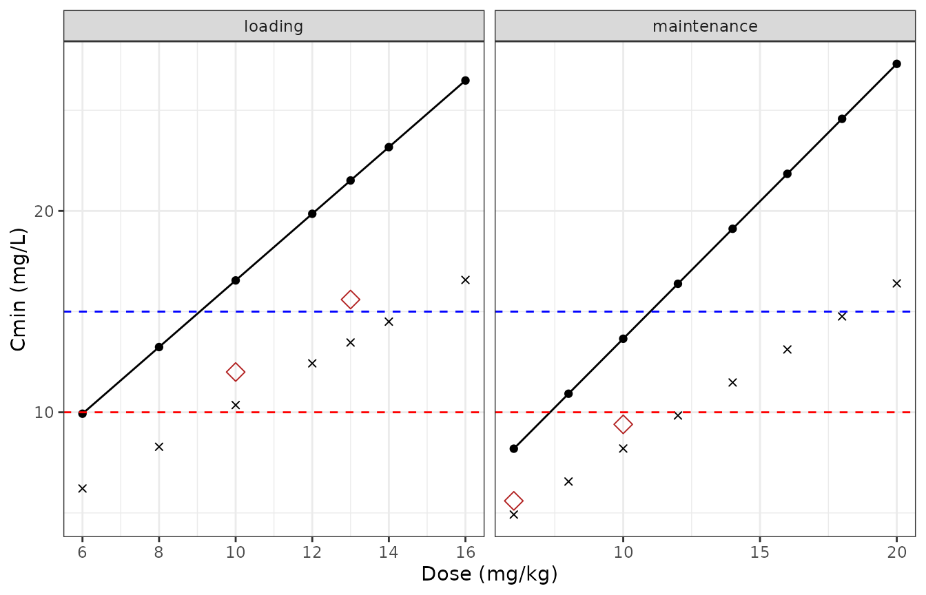
Replicates Figure 4A and 4B of Zhang 2020: mean (point) and median (cross) simulated trough by dose. The dashed lines mark the 10 and 15 mg/L targets; the open diamonds are the means the paper quotes in the text.
Comparison with the paper
The paper reports its simulations in two ways: the mean trough per regimen (Results) and the percentage of children reaching each target (Supplementary Material, Figures S1 and S2). Both are compared below.
cell <- function(tp, d, col) {
  v <- arm_summary[[col]][arm_summary$type == tp & arm_summary$mgkg == d]
  if (length(v) != 1L) stop("no unique row for ", tp, " ", d)
  v
}

cmp <- tibble::tribble(
  ~Claim,                                     ~tp,           ~d, ~col,     ~Paper,
  "Mean Cmin, loading 10 mg/kg (mg/L)",       "loading",     10, "mean",   12.0,
  "Mean Cmin, loading 13 mg/kg (mg/L)",       "loading",     13, "mean",   15.6,
  "Mean Cmin, maintenance 6 mg/kg (mg/L)",    "maintenance", 6,  "mean",   5.6,
  "Mean Cmin, maintenance 10 mg/kg (mg/L)",   "maintenance", 10, "mean",   9.4,
  "% >= 10 mg/L, loading 10 mg/kg",           "loading",     10, "p_ge10", 50.4,
  "% >= 15 mg/L, loading 10 mg/kg",           "loading",     10, "p_ge15", 26.4,
  "% >= 10 mg/L, maintenance 6 mg/kg",        "maintenance", 6,  "p_ge10", 11.1,
  "% >= 10 mg/L, maintenance 10 mg/kg",       "maintenance", 10, "p_ge10", 34.5,
  "% >= 10 mg/L, maintenance 12 mg/kg",       "maintenance", 12, "p_ge10", 45.8,
  "% >= 15 mg/L, maintenance 16 mg/kg",       "maintenance", 16, "p_ge15", 38.4
) |>
  rowwise() |>
  mutate(Simulated = cell(tp, d, col)) |>
  ungroup() |>
  mutate(Difference = Simulated - Paper)

cmp |>
  select(Claim, Paper, Simulated, Difference) |>
knitr::kable(digits = 1, caption = "Paper vs simulation. Percentages are percentage points.")| Claim | Paper | Simulated | Difference |
|---|---|---|---|
| Mean Cmin, loading 10 mg/kg (mg/L) | 12.0 | 16.5 | 4.5 |
| Mean Cmin, loading 13 mg/kg (mg/L) | 15.6 | 21.5 | 5.9 |
| Mean Cmin, maintenance 6 mg/kg (mg/L) | 5.6 | 8.2 | 2.6 |
| Mean Cmin, maintenance 10 mg/kg (mg/L) | 9.4 | 13.7 | 4.3 |
| % >= 10 mg/L, loading 10 mg/kg | 50.4 | 50.5 | 0.1 |
| % >= 15 mg/L, loading 10 mg/kg | 26.4 | 38.0 | 11.6 |
| % >= 10 mg/L, maintenance 6 mg/kg | 11.1 | 28.5 | 17.4 |
| % >= 10 mg/L, maintenance 10 mg/kg | 34.5 | 41.5 | 7.0 |
| % >= 10 mg/L, maintenance 12 mg/kg | 45.8 | 49.5 | 3.7 |
| % >= 15 mg/L, maintenance 16 mg/kg | 38.4 | 44.0 | 5.6 |
The centre of the trough distribution is reproduced: the paper reports that 50.4% of children reach 10 mg/L on the standard 10 mg/kg loading regimen, so its median trough is about 10 mg/L. On the lattice the figure is 50.5%. For 12 mg/kg maintenance the paper gives 45.8% and the lattice gives 49.5%. The ratio of the loading-regimen trough to the maintenance-regimen trough at the same mg/kg also matches: 1.26 here against 12.0 / 9.4 = 1.28 in the paper. That ratio depends only on the elimination rates, not on the dose or on the volume scale.
The spread is not reproduced. Relative to the paper, the packaged model gives a wider trough distribution: means 38-46% higher, more children above 15 mg/L, and more children above 60 mg/L (the paper reports under 2% across all regimens). The paper’s figures describe a roughly log-normal trough with a log-scale SD near 0.6 (a median of 10 with a mean of 12 and 26% above 15 mg/L fit together). The model’s IIV gives about 1.0. The most likely reason is the paper’s method: it simulated from “the PK parameters obtained from final model of each patient”, that is, from the 159 patients’ post-hoc estimates. With shrinkage of 26.9% on CL and 19.8% on Vd those estimates are narrower than the population distribution. Shrinking the lattice etas by those fractions brings the means within about 20% of the paper, but it cannot remove the difference entirely, because the patients’ own weights and creatinine values are not available. The model reproduces the paper’s parameter table. The differences are kept visible here and are not tuned away.
cmin_ratio <- cell("loading", 10, "median") / cell("maintenance", 10, "median")
cmin_ratio
#> [1] 1.263182

# All quantities are deterministic (lattice, no RNG), so these bounds do not
# depend on the machine. Measured: 50.5% / 49.5% / 1.263.
stopifnot(
  # Median: the paper's 50.4% crossing puts its median at ~10 mg/L. A 10x
  # CL or V error, or a mg/kg-vs-mg dose error, moves this by tens of points.
  abs(cell("loading", 10, "p_ge10") - 50.4) < 10,
  abs(cell("maintenance", 12, "p_ge10") - 45.8) < 10,
  # Elimination-rate check, independent of dose and volume scale.
  abs(cmin_ratio / (12.0 / 9.4) - 1) < 0.10,
  # Linearity: the paper's 15.6/12.0 and 9.4/5.6 are dose-proportional.
  abs(cell("loading", 13, "mean") / cell("loading", 10, "mean") - 1.3) < 1e-6,
  abs(cell("maintenance", 10, "mean") / cell("maintenance", 6, "mean") - 10 / 6) < 1e-6
)
Recommended regimens (Table 3, overall row)
tibble::tribble(
  ~Target,                 ~`Paper recommendation`,  ~`Simulated mean at that dose (mg/L)`, ~`Simulated median (mg/L)`,
  "Cmin >= 10, loading",   "10 mg/kg q12h x 3", cell("loading", 10, "mean"),     cell("loading", 10, "median"),
  "Cmin >= 15, loading",   "13 mg/kg q12h x 3", cell("loading", 13, "mean"),     cell("loading", 13, "median"),
  "Cmin >= 10, maintenance", "12 mg/kg q24h",   cell("maintenance", 12, "mean"), cell("maintenance", 12, "median"),
  "Cmin >= 15, maintenance", "16 mg/kg q24h",   cell("maintenance", 16, "mean"), cell("maintenance", 16, "median")
) |>
knitr::kable(digits = 1, caption = "Zhang 2020 Table 3 overall recommendations against the simulation.")| Target | Paper recommendation | Simulated mean at that dose (mg/L) | Simulated median (mg/L) |
|---|---|---|---|
| Cmin >= 10, loading | 10 mg/kg q12h x 3 | 16.5 | 10.4 |
| Cmin >= 15, loading | 13 mg/kg q12h x 3 | 21.5 | 13.5 |
| Cmin >= 10, maintenance | 12 mg/kg q24h | 16.4 | 9.8 |
| Cmin >= 15, maintenance | 16 mg/kg q24h | 21.8 | 13.1 |
The paper’s criterion was a mean trough at or above the target. Because the model’s spread is wider, the mean at every recommended dose is well above the target, and the median is at or somewhat below it. Applied to this simulation, the paper’s mean criterion would therefore pick lower doses than Table 3 does (for example, 8 rather than 10 mg/kg for the loading regimen).
NCA validation (PKNCA)
Zhang 2020 reports no NCA parameters. It computes the steady-state
exposure as AUC24 = Daily dose / CL. The check below
simulates 10 and 12 mg/kg q24h to steady state on the lattice cohort,
computes the dosing-interval AUC with PKNCA, and compares it with the
paper’s formula for each child.
The typical half-life is about 7 h, but the slowest child on the lattice has a half-life near 105 h. So the run-in to steady state is sized from that tail and not from the typical value: 50 daily doses (1,200 h) leave that child within 0.05% of steady state.
t_ss <- 1200
ss_times <- sort(unique(c(t_ss, seq(t_ss + 0.05, t_ss + 1, by = 0.05),
                          seq(t_ss + 1.25, t_ss + 24, by = 0.25))))
nca_sim <- bind_rows(lapply(c(10, 12), function(d) {
  ev <- make_events(cohort, d, seq(0, t_ss, by = 24), ss_times)
  solve_fixed(mod_typ, ev, returnType = "data.frame", addDosing = FALSE,
              rtol = 1e-10, atol = 1e-12) |>
    mutate(treatment = paste0(d, " mg/kg q24h"), mgkg = d)
}))
#> ℹ omega/sigma items treated as zero: 'etalcl', 'etalvc'
#> ℹ omega/sigma items treated as zero: 'etalcl', 'etalvc'

stopifnot(all(nca_sim$Cc >= -1e-6 * max(nca_sim$Cc)))

nca_conc <- nca_sim |>
  filter(!is.na(Cc)) |>
  mutate(Cc = pmax(Cc, 0)) |>
  select(id, treatment, time, Cc)

nca_dose <- nca_sim |>
  distinct(id, treatment, mgkg) |>
  left_join(cohort |> select(id, WT), by = "id") |>
  mutate(time = t_ss, amt = mgkg * WT)

o_conc <- PKNCAconc(nca_conc, Cc ~ time | treatment + id)
o_dose <- PKNCAdose(nca_dose, amt ~ time | treatment + id)
o_data <- PKNCAdata(
  o_conc, o_dose,
  intervals = data.frame(start = t_ss, end = t_ss + 24, auclast = TRUE, cmax = TRUE, cmin = TRUE)
)
res_nca <- suppressWarnings(pk.nca(o_data))

nca_wide <- as.data.frame(res_nca) |>
  select(treatment, id, PPTESTCD, PPORRES) |>
  pivot_wider(names_from = PPTESTCD, values_from = PPORRES)

auc_chk <- nca_wide |>
  left_join(nca_sim |> distinct(id, treatment, cl), by = c("id", "treatment")) |>
  left_join(nca_dose |> select(id, treatment, amt), by = c("id", "treatment")) |>
  mutate(auc_formula = amt / cl, pct_diff = 100 * (auclast - auc_formula) / auc_formula)

auc_chk |>
  group_by(treatment) |>
  summarise(
    `Median Cmax (mg/L)` = median(cmax),
    `Median Cmin (mg/L)` = median(cmin),
    `Median AUC24, PKNCA (mg*h/L)` = median(auclast),
    `Median AUC24, Dose/CL (mg*h/L)` = median(auc_formula),
    `Max abs % difference` = max(abs(pct_diff)),
    .groups = "drop"
  ) |>
  rename(Treatment = treatment) |>
knitr::kable(digits = 2, caption = "Steady-state NCA (1200-1224 h) against the paper's AUC24 = Dose/CL.")| Treatment | Median Cmax (mg/L) | Median Cmin (mg/L) | Median AUC24, PKNCA (mg*h/L) | Median AUC24, Dose/CL (mg*h/L) | Max abs % difference |
|---|---|---|---|---|---|
| 10 mg/kg q24h | 77.22 | 8.20 | 673.41 | 673.42 | 0.03 |
| 12 mg/kg q24h | 92.66 | 9.84 | 808.09 | 808.10 | 0.03 |
# Same drawn parameters on both sides, so this is a numerical identity. PKNCA's
# linear-up/log-down trapezoid on a 0.05-0.25 h grid is the only error source.
stopifnot(
  nrow(auc_chk) == 2 * n_arm,
  max(abs(auc_chk$pct_diff)) < 0.5
)
The AUC at steady state equals Daily dose / CL for every
child, confirming the clearance equation and the dose units. The cohort
median is also dose proportional between 10 and 12 mg/kg. The paper’s
cumulative-fraction-of-response analysis (Figures 4C, 4D and 7) weights
these AUCs by an EUCAST MRSA MIC distribution that the paper does not
print, so it is not reproduced here.
Assumptions and deviations
- Covariate form. The printed equations show theta2 and theta3 as bases raised to the covariate ratio. A secondary review that tabulated this model could not tell from its own transcription whether they were bases or exponents. The original equation image is unambiguous, and the paper’s three derived quantities (0.014 L/h/kg, 0.15 L/kg, 0.784 L/h at 70 kg) reproduce only under the base reading.
- Abstract typo. The Abstract gives clearance as “0.694 L/h”. Table 2, the equation and the Abstract’s own 0.784 L/h/70 kg all require 0.0694 L/h.
-
Typical values anchored at zero.
lclandlvcare the clearance and volume at WT = 0 (and SCr = 0), as printed. They are not the values for a typical child, which are 0.234 L/h and 2.43 L. - Residual error. The Results say an additive residual model was selected, but Table 2 reports it as “CV-sigma 7.0%”. A CV is proportional in the linear scale, and a 7.0 mg/L additive SD is ruled out by Figure 3: at a median near 10 mg/L it would push the lower 5th-percentile band well below zero, whereas the published band stays at 0-5 mg/L. The residual is therefore implemented as 7% proportional, the linear-scale equivalent of an additive error on log-transformed data.
-
IIV scale. Table 2 reports IIV as CV% with no
confidence interval, equation exponent or variance column that would
identify the convention. The CV was converted with
omega^2 = log(1 + CV^2). Reading it instead asomega = CVwould widen the distribution further, away from the paper’s simulations. - Infusion duration. Not reported. A 0.5-h infusion is used in every simulation. With a half-life of about 7 h this has little effect on the trough.
- Virtual cohort. Weight and creatinine are log-normal, matched to the Table 1 median and mean and truncated to the observed range. Their 0.5 correlation is an assumption. Age is not needed because it is not in the model.
- Simulation spread. The model’s full IIV gives a wider trough distribution than the paper’s simulations, probably because the paper sampled its patients’ post-hoc estimates. The comparison above reports the difference. It is not tuned away.
- CFR analysis not reproduced. The EUCAST MIC distribution used for Figures 4C, 4D and 7 is not printed in the paper.