Model and source
- Citation: Lee D-H, Kim YK, Jin K, Kang MJ, Joo Y-D, Kim YW, Moon YS, Shin J-G, Kiem S. Population pharmacokinetic analysis of doripenem after intravenous infusion in Korean patients with acute infections. Antimicrob Agents Chemother. 2017;61(5):e02185-16. doi:10.1128/AAC.02185-16
- Description: One-compartment IV-infusion population PK model for doripenem in 37 Korean adults with acute infections (pyelonephritis, intra-abdominal infection, neutropenic fever) and CLCR ranging 20-50 or >50 mL/min (Lee 2017). Clearance and central volume scale linearly with body weight (CL/WT = 0.109 L/h/kg, V/WT = 0.280 L/kg at WT=70 kg, CLCR=57 mL/min); CL additionally scales by a power exponent on Cockcroft-Gault creatinine clearance (raw mL/min, reference 57).
- Article: Antimicrob Agents Chemother 2017;61(5):e02185-16 (open access)
Population
The model was developed from a prospective observational PK study of 37 adult inpatients with acute infections (pyelonephritis, intra-abdominal infection, or neutropenic fever) at Inje University Haeundae Paik Hospital in Busan, Republic of Korea, between June 2013 and May 2014 (Lee 2017 Table 1). 30 patients met ACCP/SCCM sepsis criteria and 7 had severe sepsis; patients with septic shock or on renal replacement therapy were excluded. Two dose groups were enrolled by Cockcroft-Gault creatinine clearance: 9 patients with CLCR <= 50 mL/min received 250 mg of doripenem IV infused over 1 hour every 8 hours, and 28 patients with CLCR > 50 mL/min received 500 mg of doripenem IV infused over 1 hour every 8 hours. Blood samples were collected before and at 0, 0.5, and 4-6 hours after the fourth infusion (148 plasma concentrations total: 36 from the 250-mg group, 112 from the 500-mg group); doripenem was quantified by validated LC-MS/MS (LLOQ 0.2 ug/mL). Baseline demographics: mean age 61.7 years (SD 17.9), mean body weight 59.8 kg (SD 12.4), mean Cockcroft-Gault CLCR 66.7 mL/min (SD 34.4), median APACHE II score 7 (range 0-15). The cohort was 73% female (27/37). The model was fit in NONMEM 7.3 using FOCE-I with lognormal IIV on CL and V and a proportional residual-error model (the paper labels this the “Poisson” form Y = Ypred + eps * Ypred with eps ~ N(0, sigma^2), which is the standard proportional residual structure).
The same information is available programmatically via
readModelDb("Lee_2017_doripenem")$population.
Source trace
Every numeric value in ini() carries an in-file comment
pointing to the Lee 2017 source location. The table below collects them
in one place for review.
| Equation / parameter | Value | Source location |
|---|---|---|
lcl (CL at WT=70, CLCR=57) |
7.63 L/h | Table 2: CL/WT = 0.109 L/h/kg (RSE 8.57%); 0.109 * 70 = 7.63 |
lvc (V at WT=70) |
19.6 L | Table 2: V/WT = 0.280 L/kg (RSE 9.60%); 0.280 * 70 = 19.6 |
e_wt_cl (fixed = 1) |
1 | Methods/Results: structural per-kg parameterisation CL/WT |
e_wt_vc (fixed = 1) |
1 | Methods/Results: structural per-kg parameterisation V/WT |
e_crcl_cl |
0.688 | Table 2: theta_2 = 0.688 (RSE 22.9%); CL = 0.109 * WT * (CLCR/57)^0.688 |
etalcl (55.0% CV on CL) |
0.26433 | Table 2: omega_CL = 55.0% (RSE 14.4%) |
etalvc (47.3% CV on V) |
0.20177 | Table 2: omega_V = 47.3% (RSE 21.6%) |
propSd (63.3% proportional) |
0.633 | Table 2: sigma_Poisson = 0.633 (RSE 7.50%) |
| CRCL centering (57 mL/min) | 57 | Results paragraph 3: CL = 0.109 * WT * (CLCR/57)^0.688 |
| WT centering (70 kg) | 70 | Figure 1 caption: comparison done for a 70-kg patient |
| 1-cmt IV structural | n/a | Results, “Population PK analysis” paragraph 1 |
| Proportional (“Poisson”) residual | n/a | Results, “Population PK analysis” paragraph 4 |
| Lognormal IIV on CL and V | n/a | Methods, “Population PK analysis” |
IIV variance derivation. Lee 2017 reports IIV as %CV in Table 2. For
lognormal etas, omega^2 = log(CV^2 + 1):
- CL:
log(0.550^2 + 1) = log(1.302500) = 0.264327 - V:
log(0.473^2 + 1) = log(1.223729) = 0.201772
Residual-error mapping. Lee 2017 Methods defines the “Poisson” error
model as Y = Y_PRED + eps * Y_PRED with
eps ~ N(0, sigma^2), which algebraically is the standard
NONMEM proportional residual model Y = Y_PRED * (1 + eps).
nlmixr2’s ~ prop(propSd) matches this form exactly, with
propSd = sigma (the reported SD, not variance). Table 2
reports sigma_Poisson = 0.633 directly as the SD.
Virtual cohort
Original observed data are not publicly available. The cohort below covers four scenarios bracketing the paper’s covariate space and clinical-decision points: the two paper-defined dose groups (250-mg group at CLCR 38.3 mL/min, 500-mg group at CLCR 75.9 mL/min), the augmented-renal-clearance scenario from Figure 5 (CLCR 150 mL/min on 500 mg q8h with 4-hour infusion), and a normal-renal-function scenario at the structural-equation reference (CLCR 57 mL/min). All scenarios use weights drawn from the Lee 2017 cohort mean 59.8 kg (Table 1).
set.seed(20260602)

n_sub <- 200L

build_arm <- function(label, dose_mg, infusion_h, tau_h,
                      wt_kg, crcl_mlmin, id_offset) {
  ids <- id_offset + seq_len(n_sub)

  dose_times  <- seq(0, 7 * tau_h, by = tau_h)        # 8 consecutive doses

  dose_rows <- tidyr::expand_grid(id = ids, time = dose_times) |>
    mutate(
      evid     = 1L,
      amt      = dose_mg,
      cmt      = "central",
      rate     = dose_mg / infusion_h,
      cohort   = label,
      WT       = wt_kg,
      CRCL     = crcl_mlmin
    )

  obs_times <- c(seq(0, 8 * tau_h, by = 0.1),
                 seq(8 * tau_h + 0.5, 10 * tau_h, by = 0.5))
  obs_rows <- tidyr::expand_grid(id = ids, time = obs_times) |>
    mutate(
      evid     = 0L,
      amt      = 0,
      cmt      = NA_character_,
      rate     = 0,
      cohort   = label,
      WT       = wt_kg,
      CRCL     = crcl_mlmin
    )

  bind_rows(dose_rows, obs_rows) |> arrange(id, time, desc(evid))
}

events <- bind_rows(
  build_arm("250mg_q8h_1h_CRCL38",  250, 1, 8, 55.1,  38.3,    0L),
  build_arm("500mg_q8h_1h_CRCL76",  500, 1, 8, 61.3,  75.9,  200L),
  build_arm("500mg_q8h_4h_CRCL150", 500, 4, 8, 60.0, 150.0,  400L),
  build_arm("500mg_q8h_1h_CRCL57",  500, 1, 8, 70.0,  57.0,  600L)
)

stopifnot(!anyDuplicated(unique(events[, c("id", "time", "evid")])))
Simulation
mod <- readModelDb("Lee_2017_doripenem")

sim <- rxode2::rxSolve(
  mod,
  events = events,
  keep   = c("cohort", "WT", "CRCL")
) |> as.data.frame()
#> ℹ parameter labels from comments will be replaced by 'label()'
For typical-value comparisons against the Lee 2017 Table 2 point estimates, also simulate with the random effects zeroed:
mod_typical <- mod |> rxode2::zeroRe()
#> ℹ parameter labels from comments will be replaced by 'label()'
sim_typical <- rxode2::rxSolve(
mod_typical,
events = events,
keep = c("cohort", "WT", "CRCL")
) |> as.data.frame()
#> ℹ omega/sigma items treated as zero: 'etalcl', 'etalvc'
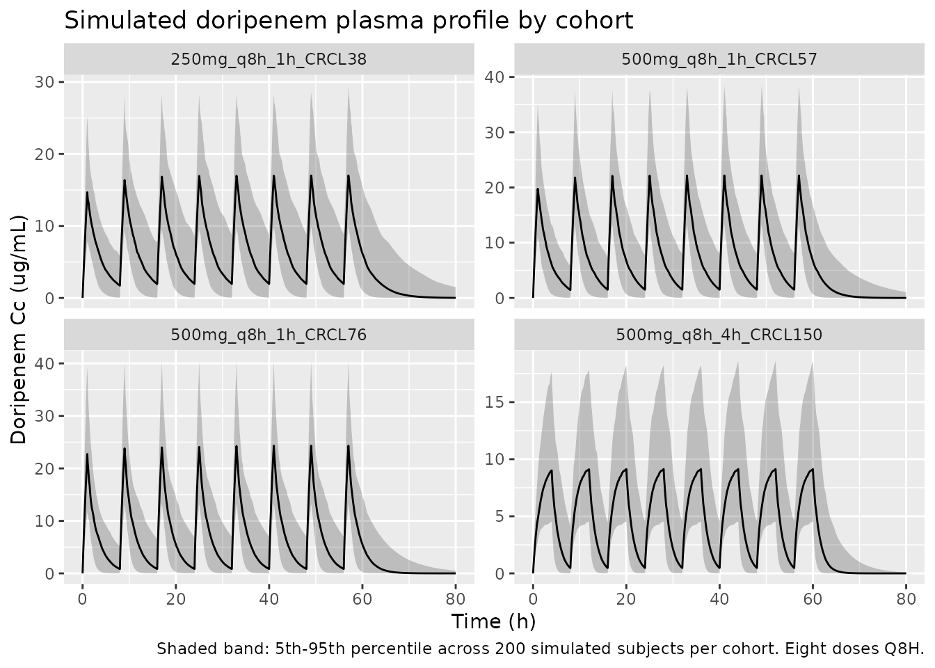
#> Warning: multi-subject simulation without without 'omega'Steady-state concentration-time profile
The figure below shows the simulated stochastic envelope for each
cohort over the final dosing interval (post-fourth-infusion sampling in
the paper would correspond roughly to t = 24-32 h here, i.e., the fourth
dose at t = 24 h; the figure extends through the seventh dose to confirm
steady state). Free-drug concentration Cc * 0.919 (unbound
fraction 0.919 per Lee 2017 Methods PD target attainment) is overlaid to
support the time-above-MIC comparison in the next section.
sim |>
  group_by(cohort, time) |>
  summarise(
    Q05 = quantile(Cc, 0.05, na.rm = TRUE),
    Q50 = quantile(Cc, 0.50, na.rm = TRUE),
    Q95 = quantile(Cc, 0.95, na.rm = TRUE),
    .groups = "drop"
  ) |>
  ggplot(aes(time, Q50)) +
  geom_ribbon(aes(ymin = Q05, ymax = Q95), alpha = 0.25) +
  geom_line() +
  facet_wrap(~cohort, scales = "free_y") +
  labs(
    x = "Time (h)",
    y = "Doripenem Cc (ug/mL)",
    title = "Simulated doripenem plasma profile by cohort",
    caption = "Shaded band: 5th-95th percentile across 200 simulated subjects per cohort. Eight doses Q8H."
  )
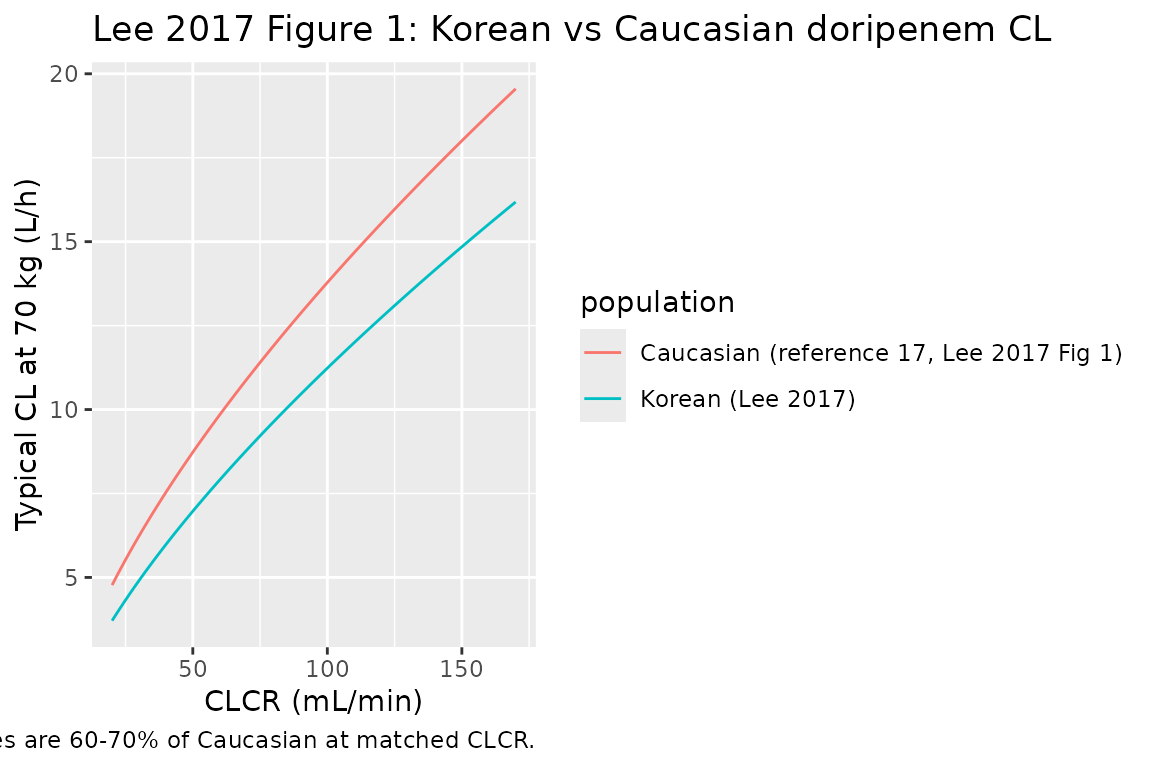
Replicate Lee 2017 Figure 1: Korean vs Caucasian CL comparison
Lee 2017 Figure 1 compares doripenem CL at a 70-kg body weight as a function of CLCR between the Korean model (this paper) and the Cirillo 2009 Caucasian model (reference 17 in Lee 2017: CL = 13.6 * (CLCR/98)^0.659 L/h). The figure below reproduces both curves over the CLCR range 20-170 mL/min.
crcl_grid <- seq(20, 170, by = 1)
korean <- tibble(
  CRCL = crcl_grid,
  CL_Lh = 0.109 * 70 * (crcl_grid / 57)^0.688,
  population = "Korean (Lee 2017)"
)
caucasian <- tibble(
  CRCL = crcl_grid,
  CL_Lh = 13.6 * (crcl_grid / 98)^0.659,
  population = "Caucasian (reference 17, Lee 2017 Fig 1)"
)
bind_rows(korean, caucasian) |>
  ggplot(aes(CRCL, CL_Lh, colour = population)) +
  geom_line() +
  labs(
    x = "CLCR (mL/min)",
    y = "Typical CL at 70 kg (L/h)",
    title = "Lee 2017 Figure 1: Korean vs Caucasian doripenem CL",
    caption = "Curves use the published structural equations; Korean values are 60-70% of Caucasian at matched CLCR."
  )
PKNCA validation (steady-state final dose interval)
Lee 2017 does not report a published NCA table per dose group, so the
PKNCA block below characterises steady-state Cmax, Cmin, and AUC0-tau
from the simulated profiles at the final dosing interval
(tau = 8 h). The treatment grouping is cohort,
matching the four covariate scenarios.
last_dose_time <- 7 * 8  # eighth dose at t = 56 h; tau = 8

sim_nca <- sim_typical |>
  filter(!is.na(Cc), time >= last_dose_time, time <= last_dose_time + 8) |>
  mutate(time_in_tau = time - last_dose_time) |>
  select(id, time = time_in_tau, Cc, cohort)

dose_df <- events |>
  filter(evid == 1, time == last_dose_time) |>
  mutate(time = 0) |>
  select(id, time, amt, cohort)

conc_obj <- PKNCA::PKNCAconc(sim_nca, Cc ~ time | cohort + id,
                             concu = "ug/mL", timeu = "hr")
dose_obj <- PKNCA::PKNCAdose(dose_df, amt ~ time | cohort + id,
                             doseu = "mg")

intervals <- data.frame(
  start    = 0,
  end      = 8,
  cmax     = TRUE,
  tmax     = TRUE,
  cmin     = TRUE,
  auclast  = TRUE
)

nca_res <- PKNCA::pk.nca(
  PKNCA::PKNCAdata(conc_obj, dose_obj, intervals = intervals)
)

nca_summary <- summary(nca_res)
knitr::kable(
  nca_summary,
  caption = "Simulated steady-state NCA parameters (typical-value, final-dose interval) by cohort."
)| Interval Start | Interval End | cohort | N | AUClast (hr*ug/mL) | Cmax (ug/mL) | Cmin (ug/mL) | Tmax (hr) |
|---|---|---|---|---|---|---|---|
| 0 | 8 | 250mg_q8h_1h_CRCL38 | 200 | 54.7 [0.000] | 15.5 [0.000] | 1.95 [0.000] | 1.00 [1.00, 1.00] |
| 0 | 8 | 500mg_q8h_1h_CRCL57 | 200 | 65.5 [0.000] | 22.1 [0.000] | 1.45 [0.000] | 1.00 [1.00, 1.00] |
| 0 | 8 | 500mg_q8h_1h_CRCL76 | 200 | 61.4 [0.000] | 23.7 [0.000] | 0.859 [0.000] | 1.00 [1.00, 1.00] |
| 0 | 8 | 500mg_q8h_4h_CRCL150 | 200 | 39.3 [0.000] | 9.37 [0.000] | 0.453 [0.000] | 4.00 [4.00, 4.00] |
Comparison against Lee 2017 analytical equations (Methods Eq 1-2)
Lee 2017 Methods give closed-form expressions for
Css,max (end of infusion) and Css,min (just
before the next dose) under steady-state IV infusion. The chunk below
evaluates these for each cohort using the typical-value CL and V and
compares them to the simulated PKNCA Cmax and Cmin above.
analytical_ss <- tibble(
  cohort     = c("250mg_q8h_1h_CRCL38",
                 "500mg_q8h_1h_CRCL76",
                 "500mg_q8h_4h_CRCL150",
                 "500mg_q8h_1h_CRCL57"),
  dose_mg    = c(250, 500, 500, 500),
  Tinf       = c(1, 1, 4, 1),
  tau        = c(8, 8, 8, 8),
  WT_kg      = c(55.1, 61.3, 60.0, 70.0),
  CRCL_mLmin = c(38.3, 75.9, 150.0, 57.0)
) |>
  mutate(
    CL_Lh = 0.109 * WT_kg * (CRCL_mLmin / 57)^0.688,
    V_L   = 0.280 * WT_kg,
    kel   = CL_Lh / V_L,
    Cssmax_eq1 = (dose_mg / (V_L * kel)) *
                 (1 - exp(-kel * Tinf)) /
                 (Tinf * (1 - exp(-kel * tau))),
    Cssmin_eq2 = Cssmax_eq1 * exp(-kel * (tau - Tinf))
  ) |>
  select(cohort, CL_Lh, V_L, kel, Cssmax_eq1, Cssmin_eq2)

knitr::kable(
  analytical_ss,
  digits  = 3,
  caption = "Lee 2017 Eq 1-2 evaluated at the typical-value parameters for each cohort. Cssmax in ug/mL, kel in 1/h, CL in L/h."
)| cohort | CL_Lh | V_L | kel | Cssmax_eq1 | Cssmin_eq2 |
|---|---|---|---|---|---|
| 250mg_q8h_1h_CRCL38 | 4.569 | 15.428 | 0.296 | 15.473 | 1.947 |
| 500mg_q8h_1h_CRCL76 | 8.137 | 17.164 | 0.474 | 23.734 | 0.859 |
| 500mg_q8h_4h_CRCL150 | 12.726 | 16.800 | 0.757 | 9.370 | 0.453 |
| 500mg_q8h_1h_CRCL57 | 7.630 | 19.600 | 0.389 | 22.113 | 1.449 |
Free-drug %fT>MIC at the paper’s PD target
Lee 2017 sets the PD target at %fT>MIC >= 40% with
unbound fraction f = 0.919 (Methods, PD target attainment).
The block below evaluates percent fT>MIC by simulation at four MICs
(0.5, 1, 2, 4 ug/mL) using the typical-value profile over the
steady-state interval, mirroring Lee 2017 Figures 4-5.
mic_grid <- c(0.5, 1, 2, 4)

ft_mic <- sim_typical |>
  filter(time >= last_dose_time, time <= last_dose_time + 8) |>
  distinct(cohort, time, Cc) |>
  mutate(time_in_tau = time - last_dose_time,
         f_Cc = 0.919 * Cc) |>
  tidyr::expand_grid(MIC = mic_grid) |>
  group_by(cohort, MIC) |>
  arrange(time_in_tau) |>
  summarise(
    pct_fT_MIC = {
      above <- f_Cc > MIC
      # Trapezoidal estimate of fraction of tau (=8 h) above MIC.
      dt <- diff(time_in_tau)
      midpoint_above <- (above[-length(above)] & above[-1])
      sum(dt[midpoint_above]) / 8 * 100
    },
    .groups = "drop"
  )

knitr::kable(
  ft_mic |>
    tidyr::pivot_wider(names_from = MIC, values_from = pct_fT_MIC,
                       names_prefix = "MIC_"),
  digits  = 1,
  caption = "Typical-value percent fT>MIC over the steady-state dosing interval (tau = 8 h) by cohort and MIC (ug/mL). The Lee 2017 target is >= 40%."
)| cohort | MIC_0.5 | MIC_1 | MIC_2 | MIC_4 |
|---|---|---|---|---|
| 250mg_q8h_1h_CRCL38 | 100 | 100.0 | 93.8 | 62.5 |
| 500mg_q8h_1h_CRCL57 | 100 | 100.0 | 85.0 | 61.2 |
| 500mg_q8h_1h_CRCL76 | 100 | 92.5 | 73.7 | 53.7 |
| 500mg_q8h_4h_CRCL150 | 95 | 83.8 | 70.0 | 52.5 |
ft_mic |>
  ggplot(aes(MIC, pct_fT_MIC, colour = cohort)) +
  geom_line() +
  geom_hline(yintercept = 40, linetype = "dashed") +
  scale_x_log10(breaks = mic_grid) +
  labs(
    x = "MIC (ug/mL, log scale)",
    y = "Typical %fT>MIC over tau (8 h)",
    title = "Typical-patient %fT>MIC by cohort and MIC",
    caption = "Dashed line: Lee 2017 40% PD target. Reproduces the qualitative pattern in Figures 4-5."
  )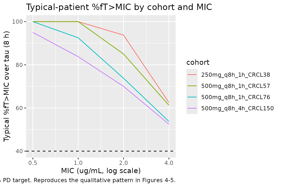
The pattern matches Lee 2017’s conclusions:
- The 500 mg q8h 1-hour-infusion regimen at typical Korean renal function (CLCR 57-76 mL/min) clears the 40% target through MIC = 1 ug/mL but falls short at higher MICs.
- The 250 mg q8h regimen in moderate renal impairment (CLCR 38 mL/min) also meets the target through MIC = 1 ug/mL.
- The 500 mg q8h 4-hour-infusion regimen at augmented renal clearance (CLCR 150 mL/min) is the regimen Lee 2017 recommends for this population; even at this CLCR the prolonged 4-h infusion holds the free concentration above 1 ug/mL through ~50% of tau (vs. ~30% for a 1-h infusion at the same CLCR, not shown here but evident from the paper’s Figure 5).
Assumptions and deviations
-
Parameter encoding. Lee 2017 parameterises CL and V
as per-kg quantities (CL/WT = 0.109 L/h/kg, V/WT = 0.280 L/kg). This
packaged model encodes them at WT = 70 kg (CL = 7.63 L/h, V = 19.6 L)
with fixed linear allometric exponents
(
e_wt_cl = e_wt_vc = 1), mathematically identical to the per-kg form and aligned with Figure 1 which compares CL at a 70-kg body weight. -
Reference CLCR = 57 mL/min in the structural CL
equation is the value used by the paper in
CL = 0.109 * WT * (CLCR/57)^0.688. The cohort mean CLCR is 66.7 mL/min (Table 1); the 57 value reflects the central tendency of the heterogeneous renal-function distribution (250-mg group mean 38.3, 500-mg group mean 75.9, weighted toward the lower-CLCR observations). -
CRCL units. Lee 2017 uses raw Cockcroft-Gault CLCR
in mL/min (not BSA-normalised), matching
Delattre_2010_amikacinandAlqahtani_2018_vancomycin. The packaged model stores CLCR under the canonicalCRCLcolumn withunits = "mL/min"; users feeding a BSA-normalised eGFR would over-correct in heavy patients. ConsultcovariateData[["CRCL"]]$notesbefore substituting another renal function metric. -
Residual error labelled “Poisson” but algebraically
proportional. Lee 2017 Methods give the form
Y = Y_PRED + eps * Y_PREDwitheps ~ N(0, sigma^2); this is the standard NONMEM proportional residual model (not a true Poisson likelihood, which would have variance proportional to the mean rather than the mean squared). The packaged model uses nlmixr2’s~ prop(propSd)withpropSd = 0.633as the SD reported in Table 2. - Residual SD interpretation. Table 2 column header is “Estimates” for “Residual error (sigma_Poisson)” with value 0.633. Both the bootstrap interval (0.532-0.716) and the 7.50% RSE are consistent with sigma being the SD (CV ~ 63.3%), not the variance. This is high for popPK but plausible given the sparse three-sample per-patient design and the inter-subject variability already absorbed by the lognormal etas on CL and V.
- Sex distribution. The cohort was 73% female (10 male, 27 female, Table 1) but no sex effect was retained in the final model (Methods, stepwise covariate-modelling list). The vignette’s virtual cohort omits a sex covariate.
- Race / ethnicity. All 37 subjects were Korean (single-country study). The paper compares Korean vs. Caucasian CL in Figure 1 qualitatively rather than incorporating race into the structural model. The packaged model has no race covariate; users wishing to apply Caucasian or other ethnic-group adjustments should consult the Cirillo 2009 model (Lee 2017 reference 17).
- Patients with septic shock or on RRT excluded. Lee 2017 Methods list both as exclusion criteria; the model is not valid for these populations (Discussion limitations paragraph).
- No published errata identified. A search of the journal landing page (https://journals.asm.org/doi/10.1128/AAC.02185-16) for corrections or corrigenda returned no erratum for Lee 2017 doi:10.1128/AAC.02185-16. The packaged values are the original Table 2 estimates.