library(nlmixr2lib)
library(PKNCA)
#>
#> Attaching package: 'PKNCA'
#> The following object is masked from 'package:stats':
#>
#>     filter
library(rxode2)
#> rxode2 5.1.8 using 2 threads (see ?getRxThreads)
#>   no cache: create with `rxCreateCache()`
library(dplyr)
#>
#> Attaching package: 'dplyr'
#> The following objects are masked from 'package:stats':
#>
#>     filter, lag
#> The following objects are masked from 'package:base':
#>
#>     intersect, setdiff, setequal, union
library(tidyr)
library(ggplot2)
Melphalan in pediatric autologous stem cell transplantation
Choi and colleagues (2026) developed a two-compartment intravenous population pharmacokinetic model for melphalan in 20 pediatric patients (age 0.6-17.4 years) undergoing autologous haematopoietic stem cell transplantation at a single Korean centre, across five different conditioning regimens. The final model carries estimated allometric body-weight exponents on clearance and both volumes, a serum-creatinine power effect on clearance, and – the paper’s main finding – a multiplicative clearance reduction when the conditioning regimen contains busulfan.
- Citation: Choi JY, Kim B, Park HJ, Kim BK, Hong KT, Lee S, Lee S, Kang HJ. Population Pharmacokinetics of Melphalan in Pediatric Patients Undergoing Autologous Hematopoietic Stem Cell Transplantation with Various Conditioning Regimens. Eur J Drug Metab Pharmacokinet. 2026;51(4):391-400. doi:10.1007/s13318-026-01000-6.
- Article: https://doi.org/10.1007/s13318-026-01000-6
- Supplement: https://doi.org/10.1007/s13318-026-01000-6 (Supplementary Information; Tables S1-S6 and Figures S1-S4)
The authors describe the model as exploratory because of the modest sample size, and the vignette below treats it that way: the validation target is the paper’s own simulation table (Table 3), which is the one published quantity the packaged model can be held to numerically.
Population
Twenty patients were enrolled prospectively between September 2020 and November 2021 (NCT04937634). Median age at melphalan infusion was 9.3 years (range 0.6-17.4), median body weight 27.6 kg (range 5.7-84.8), median body surface area 1.01 m^2 (range 0.32-2.02), and the cohort was evenly split by sex (10 female / 10 male). All patients had normal renal and hepatic function on the day of conditioning: median serum creatinine 0.51 mg/dL (range 0.34-0.67) and median eGFR (Schwartz Cr) 102.05 mL/min/1.73 m^2 (range 76.10-149.35). Baseline characteristics are Choi 2026 Table 1.
Eleven of the twenty patients received a busulfan-containing regimen – seven busulfan/melphalan (BuMel) and four busulfan/melphalan/thiotepa (BuMelThio) – and nine did not (four melphalan/etoposide/carboplatin, three BEAM, two fludarabine/melphalan). Melphalan was given as a 30-minute intravenous infusion, at 140 mg/m^2 as a single dose (BuMel, FluMel, BEAM), 50 mg/m^2 daily for two days (BuMelThio), or 140 mg/m^2 then 70 mg/m^2 on consecutive days (MEC). Sampling was five points per dosing occasion – pre-dose and 5, 40, 70 and 170 minutes after the end of infusion – giving 140 plasma samples over 28 dosing occasions. Assay LLOQ was 5 ng/mL and every post-dose sample was above it.
The same summary is available programmatically via
rxode2::rxode(readModelDb("Choi_2026_melphalan"))$population.
Source trace
The per-parameter origin is recorded as an in-file comment next to
each ini() entry in
inst/modeldb/specificDrugs/Choi_2026_melphalan.R; the table
below collects them in one place.
| Equation / parameter | Value | Source location |
|---|---|---|
| Structural model | Two-compartment, zero-order IV infusion, first-order elimination from central | Methods 2.4; Results 3.2 |
CL0 formula |
24.9 * (WT/28)^0.771 * (CREAT/0.51)^-0.686 |
Section 3.3, first displayed equation |
CLB formula |
0.846 * CL0 when the regimen contains busulfan |
Section 3.3, second displayed equation |
V1 formula |
13.4 * (WT/28)^0.872 |
Section 3.3, third displayed equation |
V2 formula |
7.37 * (WT/28)^0.553 |
Section 3.3, fourth displayed equation |
Q |
14.5 L/h (no covariate) | Table 2; Table S1 (no covariate tested on Q) |
lcl |
log(24.9) | Table 2, CL (L/h/28 kg), RSE 7.7 % |
lvc |
log(13.4) | Table 2, V1 (L/28 kg), RSE 8.7 % |
lq |
log(14.5) | Table 2, Q (L/h), RSE 22.9 % |
lvp |
log(7.37) | Table 2, V2 (L/28 kg), RSE 12.2 % |
e_wt_cl |
0.771 | Table 2, CL~WT, RSE 15.0 % |
e_wt_vc |
0.872 | Table 2, V1~WT, RSE 15.1 % |
e_wt_vp |
0.553 | Table 2, V2~WT, RSE 14.2 % |
e_creat_cl |
-0.686 | Table 2, CL~creatinine, RSE 14.7 % |
e_conmed_busulfan_cl |
0.846 | Table 2, CL~RegimenB, RSE 5.8 % |
| WT reference 28 kg | rounded-up cohort median (27.6 kg) | Table 2 footnote a |
| CREAT reference 0.51 mg/dL | cohort median | Table 1; Section 3.3 equation |
| IIV form | theta_i = theta_TV * exp(eta_i) |
Methods 2.4 |
etalcl variance |
0.279^2 = 0.077841 | Table 2, PK IIV CL (%) 27.9 |
etalvc variance |
0.399^2 = 0.159201 | Table 2, PK IIV V1 (%) 39.9 |
etalvp variance |
0.070^2 = 0.004900 | Table 2, PK IIV V2 (%) 7.0 |
cov(etalcl, etalvc) |
0.11 (correlation 0.989) | Table 2, Covariance CL~V1; supported by dOFV -38.832 in Table S2 model 4 |
propSd |
sqrt(0.0829) = 0.2879 | Table 2, Residual error Proportional (raw NONMEM variance) |
| Residual-error form | proportional only | Methods 2.4; Table S2 model 3 (combined error gave no improvement) |
Two scale readings had to be settled because Table 2 does not state
the scale of its variability rows; both are argued in full in the model
file’s ini() comments and summarised under Assumptions
and deviations below.
Virtual cohort
Individual patient data are not published. The cohort below reproduces the six simulation scenarios the authors defined in Section 2.7 and Table 3: representative South Korean paediatric body sizes at ages 0.5, 8 and 18 years (7.9, 27.5 and 66.7 kg), each crossed with presence or absence of concomitant busulfan, with serum creatinine fixed at 0.51 mg/dL and the dose computed from body surface area at 140 mg/m^2.
# Choi 2026 Table 3. Doses are the paper's own BSA-derived values.
scenarios <- tibble::tribble(
  ~scenario, ~CONMED_BUSULFAN, ~WT,  ~BSA, ~dose_mg, ~pub_cmax_ugL, ~pub_auc_ughL,
  "A",       1L,               7.9,  0.39,  53.9,    5948,          6849,
  "B",       1L,              27.5,  0.99, 138.4,    6181,          6604,
  "C",       1L,              66.7,  1.79, 251.1,    5727,          6044,
  "D",       0L,               7.9,  0.39,  53.9,    5586,          5758,
  "E",       0L,              27.5,  0.99, 138.4,    5908,          5646,
  "F",       0L,              66.7,  1.79, 251.1,    5411,          5125
)

infusion_h <- 0.5  # 30-minute IV infusion (Methods 2.2)
creat_ref  <- 0.51 # serum creatinine fixed in every scenario (Section 2.7)

knitr::kable(
  scenarios |>
    dplyr::rename(
      "Scenario"           = scenario,
      "Busulfan"           = CONMED_BUSULFAN,
      "WT (kg)"            = WT,
      "BSA (m^2)"          = BSA,
      "Dose (mg)"          = dose_mg,
      "Published Cmax (ug/L)"      = pub_cmax_ugL,
      "Published AUC0-24 (ug*h/L)" = pub_auc_ughL
    ),
  caption = "Choi 2026 Table 3 simulation scenarios and published median exposures."
)| Scenario | Busulfan | WT (kg) | BSA (m^2) | Dose (mg) | Published Cmax (ug/L) | Published AUC0-24 (ug*h/L) |
|---|---|---|---|---|---|---|
| A | 1 | 7.9 | 0.39 | 53.9 | 5948 | 6849 |
| B | 1 | 27.5 | 0.99 | 138.4 | 6181 | 6604 |
| C | 1 | 66.7 | 1.79 | 251.1 | 5727 | 6044 |
| D | 0 | 7.9 | 0.39 | 53.9 | 5586 | 5758 |
| E | 0 | 27.5 | 0.99 | 138.4 | 5908 | 5646 |
| F | 0 | 66.7 | 1.79 | 251.1 | 5411 | 5125 |
The packaged model returns Cc in mg/L (dose in mg over
volume in L), whereas Choi 2026 tabulates ug/L and ug*h/L; the
comparisons below convert the published values by dividing by 1000.
make_events <- function(scn, n, grid, id_offset = 0L) {
  subj <- tibble(
    id              = id_offset + seq_len(n),
    scenario        = scn$scenario,
    WT              = scn$WT,
    CREAT           = creat_ref,
    CONMED_BUSULFAN = scn$CONMED_BUSULFAN
  )
  dose_rows <- subj |>
    mutate(time = 0, evid = 1L, amt = scn$dose_mg,
           rate = scn$dose_mg / infusion_h, cmt = "central")
  obs_rows <- subj |>
    tidyr::crossing(time = grid) |>
    mutate(evid = 0L, amt = 0, rate = 0, cmt = "central")
  bind_rows(dose_rows, obs_rows) |>
    arrange(id, time, desc(evid))
}
Observation rows point at the central ODE state, never
at the algebraic observable Cc; referencing an observable
as a compartment renumbers the compartment slots.
Typical-value replication of Table 3
The primary numerical gate. Table 3’s medians are the paper’s own
forward simulation from this model, so a correctly transcribed model
must reproduce them. Between-subject variability is zeroed with
rxode2::zeroRe() and a dense time grid is used so the
trapezoidal AUC is not grid-limited.
mod     <- readModelDb("Choi_2026_melphalan")
mod_typ <- rxode2::zeroRe(mod)
#> ℹ parameter labels from comments will be replaced by 'label()'

grid_fine <- seq(0, 24, by = 0.01)

events_typ <- bind_rows(lapply(seq_len(nrow(scenarios)), function(i) {
  make_events(scenarios[i, ], n = 1L, grid = grid_fine, id_offset = i - 1L)
}))
stopifnot(!anyDuplicated(unique(events_typ[, c("id", "time", "evid")])))

sim_typ <- rxode2::rxSolve(
  mod_typ, events = events_typ,
  keep = c("scenario", "WT", "CONMED_BUSULFAN")
) |> as.data.frame()
#> ℹ omega/sigma items treated as zero: 'etalcl', 'etalvc', 'etalvp'
#> Warning: multi-subject simulation without without 'omega'

trapz <- function(x, y) sum(diff(x) * (head(y, -1) + tail(y, -1)) / 2)

typ_summary <- sim_typ |>
  group_by(scenario) |>
  summarise(
    cl        = first(cl),
    vc        = first(vc),
    cmax_mgL  = max(Cc),
    auc_mghL  = trapz(time, Cc),
    .groups   = "drop"
  ) |>
  left_join(
    scenarios |>
      transmute(scenario,
                pub_cmax = pub_cmax_ugL / 1000,
                pub_auc  = pub_auc_ughL / 1000),
    by = "scenario"
  ) |>
  mutate(
    cmax_pct = 100 * (cmax_mgL - pub_cmax) / pub_cmax,
    auc_pct  = 100 * (auc_mghL - pub_auc)  / pub_auc
  )

knitr::kable(
  typ_summary |>
    dplyr::rename(
      "Scenario"              = scenario,
      "CL (L/h)"              = cl,
      "V1 (L)"                = vc,
      "Cmax sim (mg/L)"       = cmax_mgL,
      "AUC0-24 sim (mg*h/L)"  = auc_mghL,
      "Cmax Table 3 (mg/L)"   = pub_cmax,
      "AUC0-24 Table 3 (mg*h/L)" = pub_auc,
      "Cmax diff (%)"         = cmax_pct,
      "AUC diff (%)"          = auc_pct
    ),
  digits = c(0, 2, 2, 3, 3, 3, 3, 2, 2),
  caption = "Typical-value simulation vs. Choi 2026 Table 3 medians."
)| Scenario | CL (L/h) | V1 (L) | Cmax sim (mg/L) | AUC0-24 sim (mg*h/L) | Cmax Table 3 (mg/L) | AUC0-24 Table 3 (mg*h/L) | Cmax diff (%) | AUC diff (%) |
|---|---|---|---|---|---|---|---|---|
| A | 7.94 | 4.45 | 5.865 | 6.787 | 5.948 | 6.849 | -1.40 | -0.90 |
| B | 20.77 | 13.19 | 6.190 | 6.662 | 6.181 | 6.604 | 0.15 | 0.88 |
| C | 41.14 | 28.56 | 5.740 | 6.104 | 5.727 | 6.044 | 0.23 | 1.00 |
| D | 9.39 | 4.45 | 5.557 | 5.742 | 5.586 | 5.758 | -0.53 | -0.27 |
| E | 24.56 | 13.19 | 5.853 | 5.636 | 5.908 | 5.646 | -0.93 | -0.18 |
| F | 48.62 | 28.56 | 5.436 | 5.164 | 5.411 | 5.125 | 0.46 | 0.77 |
# This gate is DETERMINISTIC on our side: zeroRe(), fixed covariates, fixed
# grid. The residual difference is the Monte Carlo noise of the paper's own
# 1000-draw medians. Realised max |diff| = 1.40 % (Cmax, scenario A).
# A mis-transcribed clearance, exponent, reference weight or dose moves these
# by tens of percent, so 3 % keeps the gate able to go red.
stopifnot(
  max(abs(typ_summary$cmax_pct)) < 3,
  max(abs(typ_summary$auc_pct))  < 3
)
An independent closed-form check: because the profile is essentially complete within 24 h, AUC0-24 should equal Dose / CL. This is volume-free and therefore isolates the clearance model.
closed_form <- typ_summary |>
  left_join(scenarios |> select(scenario, dose_mg), by = "scenario") |>
  mutate(auc_dose_over_cl = dose_mg / cl,
         pct = 100 * (auc_mghL - auc_dose_over_cl) / auc_dose_over_cl)

# Deterministic identity; realised max |diff| < 0.001 %. Any gap beyond ~1 %
# means the ODE is not receiving the full dose or the window is too short.
stopifnot(max(abs(closed_form$pct)) < 1)

knitr::kable(
  closed_form |>
    select(scenario, auc_mghL, auc_dose_over_cl, pct) |>
    dplyr::rename(
      "Scenario"                 = scenario,
      "AUC0-24 trapezoidal (mg*h/L)" = auc_mghL,
      "Dose / CL (mg*h/L)"       = auc_dose_over_cl,
      "Difference (%)"           = pct
    ),
  digits = c(0, 3, 3, 3),
  caption = "Trapezoidal AUC0-24 against the closed-form Dose / CL identity."
)| Scenario | AUC0-24 trapezoidal (mg*h/L) | Dose / CL (mg*h/L) | Difference (%) |
|---|---|---|---|
| A | 6.787 | 6.787 | 0 |
| B | 6.662 | 6.662 | 0 |
| C | 6.104 | 6.104 | 0 |
| D | 5.742 | 5.742 | 0 |
| E | 5.636 | 5.636 | 0 |
| F | 5.164 | 5.164 | 0 |
Covariate effect sizes
Choi 2026 reports that concomitant busulfan raises AUC0-24 by 1.17- to 1.19-fold at matched body weight, and that the lowest-weight scenario has a 1.12- to 1.13-fold higher AUC0-24 than the highest-weight scenario within a regimen group.
auc_of <- function(s) typ_summary$auc_mghL[typ_summary$scenario == s]

effects <- tibble::tribble(
  ~Comparison,                          ~Simulated,                 ~Published,
  "Busulfan vs none, 7.9 kg (A/D)",     auc_of("A") / auc_of("D"),  6849 / 5758,
  "Busulfan vs none, 27.5 kg (B/E)",    auc_of("B") / auc_of("E"),  6604 / 5646,
  "Busulfan vs none, 66.7 kg (C/F)",    auc_of("C") / auc_of("F"),  6044 / 5125,
  "7.9 vs 66.7 kg, busulfan (A/C)",     auc_of("A") / auc_of("C"),  6849 / 6044,
  "7.9 vs 66.7 kg, no busulfan (D/F)",  auc_of("D") / auc_of("F"),  5758 / 5125
)

knitr::kable(effects, digits = 4,
caption = "Simulated covariate effect on AUC0-24 vs. the ratios implied by Choi 2026 Table 3.")| Comparison | Simulated | Published |
|---|---|---|
| Busulfan vs none, 7.9 kg (A/D) | 1.1820 | 1.1895 |
| Busulfan vs none, 27.5 kg (B/E) | 1.1820 | 1.1697 |
| Busulfan vs none, 66.7 kg (C/F) | 1.1820 | 1.1793 |
| 7.9 vs 66.7 kg, busulfan (A/C) | 1.1119 | 1.1332 |
| 7.9 vs 66.7 kg, no busulfan (D/F) | 1.1119 | 1.1235 |
# The busulfan ratio is exact by construction: 1 / 0.846 = 1.1820, independent
# of weight, because the multiplier enters clearance alone. Deterministic.
stopifnot(abs(effects$Simulated[1:3] - 1 / 0.846) < 0.001)

# The weight ratio is the model's own prediction (1.1119) rather than an
# identity; the published 1.12-1.13 is a ratio of two Monte Carlo medians and
# so carries their noise. Realised gap 1.9 % (A/C) and 1.0 % (D/F). 5 %
# tolerance admits that and still catches a wrong allometric exponent, which
# would move the ratio by much more.
stopifnot(max(abs(effects$Simulated[4:5] / effects$Published[4:5] - 1)) < 0.05)
Stochastic cohort
Two hundred virtual subjects per scenario, with the published
between-subject variability and the correlated CL-V1 random effects
active. Residual error is deliberately excluded (Cc is the
individual prediction), matching the paper’s Table 3: its percentile
spreads recover the clearance IIV alone, which is what a residual-free
simulation produces.
# set.seed() seeds R's RNG, not rxode2's; rxode2 partitions its streams per
# solver thread, so the cohort drawn here differs between a 2-thread CI runner
# and a 16-thread workstation. Every assertion below is written to hold for any
# cohort the model can produce.
set.seed(20260429)

n_per_arm  <- 200L
grid_coh   <- sort(unique(c(seq(0, 3, by = 0.025), seq(3, 24, by = 0.15))))

events <- bind_rows(lapply(seq_len(nrow(scenarios)), function(i) {
  make_events(scenarios[i, ], n = n_per_arm, grid = grid_coh,
              id_offset = (i - 1L) * n_per_arm)
}))
stopifnot(!anyDuplicated(unique(events[, c("id", "time", "evid")])))

sim <- rxode2::rxSolve(
  mod, events = events,
  keep = c("scenario", "WT", "CONMED_BUSULFAN")
) |> as.data.frame()
#> ℹ parameter labels from comments will be replaced by 'label()'

stopifnot(nrow(sim) > 0, !anyNA(sim$Cc), all(sim$Cc >= 0))
Replicating Figure 2
Choi 2026 Figure 2 is a box plot of simulated Cmax and AUC0-24 across the six scenarios.
# rxSolve does not return an `evid` column -- its output holds the requested
# observation grid only, so no filtering on event type is needed (or possible).
per_subject <- sim |>
  group_by(id, scenario) |>
  summarise(
    Cmax = max(Cc) * 1000,                 # mg/L -> ug/L
    AUC  = trapz(time, Cc) * 1000,         # mg*h/L -> ug*h/L
    .groups = "drop"
  )

per_subject |>
  tidyr::pivot_longer(c(Cmax, AUC), names_to = "Parameter", values_to = "Value") |>
  mutate(Parameter = factor(Parameter, levels = c("Cmax", "AUC"),
                            labels = c("Cmax (ug/L)", "AUC0-24 (ug*h/L)"))) |>
  ggplot(aes(scenario, Value)) +
  geom_boxplot(outlier.size = 0.5) +
  facet_wrap(~Parameter, scales = "free_y") +
  labs(x = "Scenario", y = NULL,
       caption = "Compare against Choi 2026 Figure 2 and Table 3.")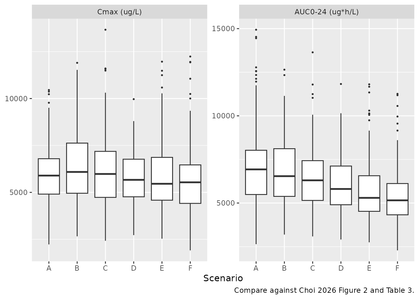
Replicates Figure 2 of Choi 2026: simulated Cmax and AUC0-24 by scenario (200 virtual subjects per arm).
The variability scale, as a live check
Table 2 prints its inter-individual variability rows under a
(%) qualifier without saying whether the numbers are
log-scale SDs or back-transformed CVs. Because AUC is inversely
proportional to clearance, the log-scale SD of the simulated AUC0-24
recovers omega_CL directly. The packaged model reads the
printed 27.9 as 100 * omega, so this statistic should
return ~0.279.
omega_from_spread <- per_subject |>
  group_by(scenario) |>
  summarise(
    sd_log_auc = (log(quantile(AUC, 0.95)) - log(quantile(AUC, 0.05))) /
      (2 * qnorm(0.95)),
    .groups = "drop"
  )

knitr::kable(
  omega_from_spread |>
    mutate(in_model = 0.279) |>
    dplyr::rename(
      "Scenario"                        = scenario,
      "omega_CL from simulated spread"  = sd_log_auc,
      "omega_CL in the model"           = in_model
    ),
  digits = 4,
  caption = "Log-scale SD of simulated AUC0-24 recovers the clearance IIV."
)| Scenario | omega_CL from simulated spread | omega_CL in the model |
|---|---|---|
| A | 0.3128 | 0.279 |
| B | 0.2838 | 0.279 |
| C | 0.2566 | 0.279 |
| D | 0.2742 | 0.279 |
| E | 0.2921 | 0.279 |
| F | 0.2544 | 0.279 |
# The same statistic applied to Choi 2026 Table 3's own 5th-95th percentiles
# gives 0.275, 0.282, 0.275, 0.287, 0.279, 0.285 -- mean 0.280 against the
# printed 27.9, which is what pinned the scale. Here it is a regression test.
# Realised 0.2544-0.3128 across the six arms (max 12.1 % from 0.279), identical
# at 2 and 16 solver threads; a 5th/95th percentile from n = 200 is noisy, so
# the bound is +/- 25 %. Reading the printed value as a CV would give 0.274
# (inside, but that reading is excluded on other grounds); reading it as a
# variance would give 0.528, and dropping the IIV entirely would give ~0 --
# both break this gate.
stopifnot(all(abs(omega_from_spread$sd_log_auc / 0.279 - 1) < 0.25))
PKNCA validation
sim_nca <- sim |>
  filter(!is.na(Cc)) |>
  select(id, time, Cc, scenario)

# Guarantee a time = 0 row per (id, scenario); plasma is zero at the start of
# an IV infusion. Filtering on `time > 0` or `Cc > 0` would drop it and trigger
# PKNCA's "AUC range starting before the first measurement" warning.
sim_nca <- bind_rows(
  sim_nca,
  sim_nca |> distinct(id, scenario) |> mutate(time = 0, Cc = 0)
) |>
  distinct(id, scenario, time, .keep_all = TRUE) |>
  arrange(id, scenario, time)

dose_df <- events |>
  filter(evid == 1) |>
  select(id, time, amt, scenario)

conc_obj <- PKNCA::PKNCAconc(sim_nca, Cc ~ time | scenario + id,
                             concu = "mg/L", timeu = "h")
dose_obj <- PKNCA::PKNCAdose(dose_df, amt ~ time | scenario + id,
                             doseu = "mg")

intervals <- data.frame(
  start   = 0,
  end     = 24,
  cmax    = TRUE,
  tmax    = TRUE,
  auclast = TRUE
)

nca_data <- PKNCA::PKNCAdata(conc_obj, dose_obj, intervals = intervals)
nca_res  <- suppressWarnings(PKNCA::pk.nca(nca_data))
Comparison against Choi 2026 Table 3
published <- scenarios |>
  transmute(scenario,
            cmax    = pub_cmax_ugL / 1000,   # ug/L    -> mg/L
            auclast = pub_auc_ughL / 1000)   # ug*h/L  -> mg*h/L

cmp <- nlmixr2lib::ncaComparisonTable(
  simulated = nca_res,
  reference = published,
  by        = "scenario",
  units     = c(cmax = "mg/L", auclast = "mg*h/L", tmax = "h"),
  tolerance_pct = 20
)

knitr::kable(
  cmp,
  caption = "Simulated vs. published NCA from Choi 2026 Table 3. * indicates >20% absolute difference from the reference value."
)| NCA parameter | scenario | Reference | Simulated | % diff |
|---|---|---|---|---|
| Cmax (mg/L) | A | 5.95 | 5.89 | -0.9% |
| Cmax (mg/L) | B | 6.18 | 6.09 | -1.5% |
| Cmax (mg/L) | C | 5.73 | 5.98 | +4.4% |
| Cmax (mg/L) | D | 5.59 | 5.67 | +1.5% |
| Cmax (mg/L) | E | 5.91 | 5.46 | -7.6% |
| Cmax (mg/L) | F | 5.41 | 5.54 | +2.3% |
| AUClast (mg*h/L) | A | 6.85 | 6.93 | +1.2% |
| AUClast (mg*h/L) | B | 6.6 | 6.54 | -1.0% |
| AUClast (mg*h/L) | C | 6.04 | 6.3 | +4.3% |
| AUClast (mg*h/L) | D | 5.76 | 5.8 | +0.8% |
| AUClast (mg*h/L) | E | 5.65 | 5.3 | -6.2% |
| AUClast (mg*h/L) | F | 5.12 | 5.15 | +0.6% |
No row is starred: every simulated median sits within 20 % of Choi 2026 Table 3. The largest gap is scenario E (-7.6 % on Cmax, -6.2 % on AUClast), which is cohort noise rather than a structural disagreement – the same scenario is reproduced to 0.9 % (Cmax) and 0.2 % (AUC) by the typical-value simulation above, where no sampling is involved.
nca_med <- as.data.frame(nca_res$result) |>
  filter(PPTESTCD %in% c("cmax", "auclast")) |>
  group_by(scenario, PPTESTCD) |>
  summarise(sim = median(PPORRES), .groups = "drop") |>
  tidyr::pivot_wider(names_from = PPTESTCD, values_from = sim) |>
  left_join(published, by = "scenario", suffix = c("_sim", "_pub")) |>
  mutate(
    cmax_pct    = 100 * (cmax_sim    - cmax_pub)    / cmax_pub,
    auclast_pct = 100 * (auclast_sim - auclast_pub) / auclast_pub
  )

# Cohort medians, so this is noisier than the typical-value gate above: the
# bound must admit the draw-to-draw spread of a 200-subject median (SE ~2.5 %
# per arm, and this takes the max over six arms) plus the coarser observation
# grid used for the cohort and the Monte Carlo noise in the paper's own
# medians. Realised max |diff| 7.6 % (Cmax, scenario E) and 6.2 % (AUClast,
# scenario E), identical at 2 and 16 solver threads. 15 % keeps headroom above
# that while still going red on a mis-transcribed parameter, which moves these
# by tens of percent.
stopifnot(
  max(abs(nca_med$cmax_pct))    < 15,
  max(abs(nca_med$auclast_pct)) < 15
)
Assumptions and deviations
-
Scale of the inter-individual variability rows (resolved,
with the competing reading recorded). Choi 2026 Table 2 prints
its IIV rows as
CL (%) 27.9,V1 (%) 39.9,V2 (%) 7.0without saying whether these are log-scale SDs (100 * omega) or back-transformed CVs (100 * sqrt(exp(omega^2) - 1)). The packaged model reads them as100 * omega. Three independent checks agree: (i) the log-scale SD of the AUC0-24 percentiles in the paper’s own Table 3 is 0.280 averaged over the six scenarios, against a printed 27.9; (ii) under the CV reading,omega_CL = 0.2737andomega_V1 = 0.3843, for which the printed covariance 0.11 implies a CL-V1 correlation of 1.046 – not a valid covariance matrix; (iii) for V1 the two readings are separable and the printed 39.9 is exactly100 * omega, where the CV would be 41.5. To adopt the CV reading instead, theini()variances would becomelog(1 + (value/100)^2). -
Scale of the residual-error row (resolved, with the
competing reading recorded). Table 2 prints
Proportional 0.0829with no qualifier. The packaged model reads it as the raw NONMEM SIGMA variance, givingpropSd = sqrt(0.0829) = 0.2879. Evidence:estimate +/- 1.96 * RSE * estimate= 0.0829 +/- 0.0167 reproduces the width of the printed bootstrap CI (0.0616-0.0946), so the RSE and the estimate share a scale – and a NONMEM RSE is on the variance scale; and the authors qualified exactly one block of Table 2 with(%)(the IIV rows), leaving the residual row as raw output. If 0.0829 were already an SD the proportional error would be 8.29 %; to adopt that reading, setpropSd <- 0.0829. This choice does not affect any validation in this vignette, because every check usesCc, the individual prediction, which carries no residual error – and the paper’s own Table 3 percentiles likewise recover the clearance IIV alone, implying its simulation was also residual-free. -
CL-V1 correlation of 0.989. Taking the printed
variances and the printed covariance 0.11 at face value gives a
near-unity correlation. The matrix remains positive definite
(eigenvalues 0.2358, 0.0049, 0.0012) and
chol()succeeds, so it is encoded verbatim with no nudge. The magnitude is corroborated by the paper’s own model-building table: adding the covariance bought dOFV = -38.832 on one degree of freedom (Table S2, model 4), which only a very strong correlation produces. -
No covariate on Q. Table 2 labels the clearance and
volume rows
/28 kgbut labels Q simplyQ (L/h), the Table 2 footnote restricts the allometric exponents to CL, V1 and V2, and Table S1 lists no covariate tested on Q. Q is therefore encoded without weight scaling, which is unusual for an allometric model and is the authors’ choice, not a transcription gap. -
Weight exponents are estimated, not fixed. 0.771 /
0.872 / 0.553 rather than the theoretical 0.75 / 1.0 / 1.0, so they are
not wrapped in
fixed(). -
Creatinine covariate support is narrow. Every
patient had normal renal function (serum creatinine 0.34-0.67 mg/dL), so
the
(CREAT/0.51)^-0.686term is only supported over that interval. Extrapolating it to renal impairment is unsupported by the source data. -
Busulfan is a carried-over regimen effect, not a concurrent
exposure. Busulfan was given on days -9 to -6 (BuMel) or -9 to
-7 (BuMelThio), finishing before the melphalan dose on day -5, -4 or -3.
The
CONMED_BUSULFANflag therefore marks regimen membership; the paper proposes regimen-related organ dysfunction and oxidative-stress pathways as mechanisms and explicitly calls the effect preliminary. -
Virtual cohort covariates are fixed, not sampled.
The paper’s Section 2.7 scenarios fix body weight, creatinine and
regimen and vary only the random effects; this vignette does the same,
so the simulated spread reflects IIV alone. That is what makes the
AUC0-24 percentile spread a clean readout of
omega_CL. - Supplement typographical error. Table S2 labels the base-model candidates “1-compartment oral” and “2-compartment oral”. Melphalan was given intravenously over 30 minutes and Methods 2.4 states the administration was modelled as a zero-order infusion; the model is encoded as IV with no depot or bioavailability term.
- No observed-vs-predicted overlay. Patient-level concentrations are available only from the corresponding author on request, so the vignette validates against the paper’s published simulation table rather than against observed data, and does not attempt to reproduce the goodness-of-fit panels of Figure 1.