6-Mercaptopurine + methotrexate maintenance therapy in childhood ALL (Gebhard 2023) • nlmixr2lib

Model and source

Gebhard et al. (2023) developed three linked models from a single cohort of 452 children on maintenance therapy for acute lymphoblastic leukemia (ALL). Each has its own final parameter table, cross-validation, goodness-of-fit plot and visual predictive check, so each is packaged as its own model file:

Model file	Paper’s model	Parameter source	Output
`Gebhard_2023_methotrexate`	`PK^MTX_{fix,bio,lin,peri}`	Table 2 + Suppl. Table S1	E-MTX
`Gebhard_2023_mercaptopurine`	`PK^6MP_{mm,pop}`	Table 3 + Suppl. Table S2	E-TGN
`Gebhard_2023_mercaptopurine_anc`	`PKPD^6MP_{lin,mm}`	Table 5 + Suppl. Table S11	E-TGN, ANC

Article: https://doi.org/10.1038/s41598-023-38414-0
Supplementary information: https://www.nature.com/articles/s41598-023-38414-0#Sec22

mod_mtx  <- rxode2::rxode(readModelDb("Gebhard_2023_methotrexate"))
mod_6mp  <- rxode2::rxode(readModelDb("Gebhard_2023_mercaptopurine"))
mod_pkpd <- rxode2::rxode(readModelDb("Gebhard_2023_mercaptopurine_anc"))

Citation: Gebhard A, Lilienthal P, Metzler M, Rauh M, Sager S, Schmiegelow K, Toksvang LN, Zierk J. (2023). Pharmacokinetic-pharmacodynamic modeling of maintenance therapy for childhood acute lymphoblastic leukemia. Sci Rep 13:11749. doi:10.1038/s41598-023-38414-0. Fixed plasma-PK parameters are reproduced in Gebhard 2023 Supplementary Table S11 from Lennard L, Keen D, Lilleyman JS (1986) and Brunton LL, Lazo JS, Parker K (2005); k_circ is fixed from Jost F, Zierk J, Le TT, et al. (2020). The myelosuppression structure is Friberg LE, Henningsson A, Maas H, Nguyen L, Karlsson MO. (2002). Model of chemotherapy-induced myelosuppression with parameter consistency across drugs. J Clin Oncol 20(24):4713-4721. doi:10.1200/JCO.2002.02.140. The 6MP-only PK arm is modellib(‘Gebhard_2023_mercaptopurine’) and the methotrexate arm is modellib(‘Gebhard_2023_methotrexate’).

The joint PKPD model is the paper’s headline result. Its superscript (PKPD^6MP) records that the effect function is driven by the erythrocyte thioguanine-nucleotide concentration E-TGN alone; the sibling variant PKPD^{6MP,MTX} that adds a slope^MTX * E-MTX term (equation PKPD7b, Supplementary Table S10) was tested and rejected. Supplementary Information section I lists only the 6MP arm and the five PD compartments, matching the Discussion’s statement that “our final PKPD model does not include a MTX PK submodel”. The methotrexate arm therefore lives in its own model file.

Population

The analysis pooled 452 children with precursor-B-cell ALL treated on the NOPHO ALL-92 protocol (Nordic Society for Paediatric Haematology and Oncology). Median age 5.9 years (range 2.4-16.9), weight 21.5 kg (10.3-105.5), height 114.0 cm (81.5-180.0). Maintenance therapy was oral 6-mercaptopurine 57.1 mg/m^2 daily (5.4-175.0) plus oral methotrexate 15.0 mg/m^2 weekly (1.3-45.0), titrated to a target white-blood-cell count of 1.5-3.5 G/L. The data set holds 4624 E-TGN, 4192 E-MTX and 9808 ANC observations (Gebhard 2023 Table 1).

Each patient’s record begins with the first paired E-TGN / E-MTX measurement taken 28 days after the last high-dose intravenous methotrexate course, so the high-dose-MTX period is excluded and every record starts mid-therapy. That single fact drives two of the model’s more unusual features: the red-cell compartments are initialised at the patient’s first observed concentration rather than at zero, and the Friberg chain is initialised at a treatment steady state scaled by an estimated fraction-of-baseline parameter inieff.

The same information is available programmatically via each model’s population metadata (readModelDb("Gebhard_2023_mercaptopurine_anc")()$population).

Source trace

The per-parameter origin is recorded as an in-file comment next to each ini() entry. The table below collects them in one place.

Equation / parameter	Value	Source location
`d/dt(depot)`, `d/dt(central)`, `d/dt(peripheral1)` (MTX)	n/a	Equations MTX1-MTX3, p. 4
`d/dt(rbc_mtx)` (linear influx from the peripheral compartment)	n/a	Equation MTX4c, p. 4
`lka` (MTX)	26.64 1/day	Suppl. Table S1
`lvc` (MTX)	11.606 L/m^2	Suppl. Table S1
`lvp` (MTX)	4.347 L/m^2	Suppl. Table S1
`lcl` (MTX)	14.2944 x 11.606 = 165.90 L/day/m^2	Suppl. Table S1 (`ke^MTX` x `V_C^MTX`)
`lq` (MTX)	0.9888 x 11.606 = 11.476 L/day/m^2	Suppl. Table S1 (`k_cp` x `V_C^MTX`)
`lfdepot` / `limax_fdepot` / `ld50_fdepot` (MTX)	1 / 0.77 / 15.01 mg/m^2	Suppl. Table S1 (`F^MTX = 1 - 0.77 MTX / (15.01 + MTX)`)
`lkinf_rbc` (MTX)	0.031 1/day	Table 2
`lkeff_rbc` (MTX)	0.018 1/day	Table 2
`etalkinf_rbc` / `etalkeff_rbc` (MTX)	CV 34% / 31%	Table 2
`addSd_Crbc_mtx` / `propSd_Crbc_mtx`	sqrt(0.000018) / sqrt(0.024)	Table 2 (read as variances; see Errata)
`d/dt(depot)`, `d/dt(central)` (6MP)	n/a	Equations 6MP1-6MP2, p. 5
`d/dt(rbc_tgn)` (Michaelis-Menten influx)	n/a	Equation 6MP3b, p. 5
`lka` / `lvc` / `lcl` / `lfdepot` (6MP)	21.07 1/day / 20.1911 L/m^2 / 15.4 x 20.1911 / 0.12	Suppl. Tables S2, S11
`lvmax_rbc` / `lkm_rbc` / `lkeff_rbc` (6MP PK only)	0.096 umol/L/day / 0.016 umol/L / 0.041 1/day	Table 3
`etalvmax_rbc` / `etalkeff_rbc` (6MP PK only)	CV 52% / 50% (no IIV on `K_mm`)	Table 3
`addSd_Crbc_tgn` / `propSd_Crbc_tgn` (6MP PK only)	sqrt(0.023) / sqrt(0.064)	Table 3
`lvmax_rbc` / `lkm_rbc` / `lkeff_rbc` (PKPD)	0.21 umol/L/day / 0.14 umol/L / 0.050 1/day	Table 5
`d/dt(precursor1..4)`, `d/dt(circ)`, `fb`	n/a	Equations PKPD1-PKPD6, p. 5
`edrug = slope * rbc_tgn`	n/a	Equation PKPD7a, p. 6
`lrbase` (`base`)	2.17 G/L	Table 5
`lktr` (`k_tr`; `k_prol` fixed equal to it)	0.15 1/day	Table 5 + main text
`lslope`	0.16 L/umol	Table 5
`lgamma`	0.79	Table 5
`linieff`	0.87	Table 5
`lkout` (`k_circ`, fixed)	2.3765 1/day	Suppl. Table S11 (Jost et al.)
IIV on the seven PKPD parameters	CV 56 / 54 / 27 / 72 / 81 / 11 / 54 %	Table 5
`addSd_Crbc_tgn` / `propSd_Crbc_tgn` / `propSd_ANC` (PKPD)	sqrt(0.024) / sqrt(0.061) / sqrt(0.25)	Table 5
Initial conditions `X_E(0) = INITGN`, `X_ma(0) = inieff * base`	n/a	Suppl. Information section I

Units and dosing convention

Gebhard 2023 states that the observations were converted to umol/L (assuming a hemoglobin molecular weight of 64458 g/mol and 330 g Hb/L erythrocytes) but never states the units of the plasma concentrations. They are pinned by dimensional analysis. In equation MTX4c, dX_E/dt = K_in (X_P / V_P) - K_eff X_E, both K_in and K_eff are reported in 1/day, so for K_in * C_plasma to carry the units of dX_E/dt (umol/L/day), C_plasma must be in umol/L. Equation 6MP3b gives the same answer independently: K_mm is reported in umol/L and is added directly to the plasma concentration in the denominator.

Volumes are per m^2 body-surface area, so doses must be supplied in umol/m^2 – BSA cancels out of the model entirely and no BSA covariate is needed. Clinical mg/m^2 doses convert with the molecular weights below. That conversion is a derived quantity, not printed in the paper.

MW_MTX <- 454.44   # g/mol, methotrexate
MW_6MP <- 152.18   # g/mol, 6-mercaptopurine

umol_m2 <- function(mg_m2, mw) mg_m2 * 1000 / mw

MTX_DOSE_MGM2 <- 15.0   # median weekly dose, Table 1
MP_DOSE_MGM2  <- 57.1   # median daily  dose, Table 1

c(MTX = umol_m2(MTX_DOSE_MGM2, MW_MTX), MP = umol_m2(MP_DOSE_MGM2, MW_6MP))
#>       MTX        MP 
#>  33.00766 375.21356

Structural identity checks

Before any simulation, the reparameterisation from the paper’s micro-constants to the library’s canonical lcl / lq / lvc / lvp is checked against the paper’s own printed numbers. These are exact algebraic identities, so they are asserted rather than eyeballed.

mtx <- mod_mtx$theta    # methotrexate PK model
mp6 <- mod_6mp$theta    # 6MP PK-only model
mp  <- mod_pkpd$theta   # joint PKPD model

vc_mtx <- exp(mtx[["lvc"]]); vp_mtx <- exp(mtx[["lvp"]])
cl_mtx <- exp(mtx[["lcl"]]); q_mtx  <- exp(mtx[["lq"]])

structural <- tibble::tibble(
  Quantity = c(
    "ke^MTX = CL / V_C (1/day)",
    "k_cp = Q / V_C (1/day)",
    "k_pc = Q / V_P (1/day)",
    "V_P = V_C k_cp / k_pc (L/m^2)",
    "ke^6MP = CL / V_C (1/day)",
    "mature-neutrophil half-life ln(2) / k_circ (day)",
    "F^MTX at the median 15 mg/m^2 weekly dose"
  ),
  Model = c(
    cl_mtx / vc_mtx,
    q_mtx / vc_mtx,
    q_mtx / vp_mtx,
    vc_mtx * (q_mtx / vc_mtx) / (q_mtx / vp_mtx),
    exp(mp[["lcl"]]) / exp(mp[["lvc"]]),
    log(2) / exp(mp[["lkout"]]),
    1 - exp(mtx[["limax_fdepot"]]) * MTX_DOSE_MGM2 /
      (exp(mtx[["ld50_fdepot"]]) + MTX_DOSE_MGM2)
  ),
  Paper = c(14.2944, 0.9888, 2.64, 4.347, 15.4, 0.29, 0.6151),
  Source = c(
    "Suppl. Table S1", "Suppl. Table S1", "Suppl. Table S1",
    "Suppl. Table S1", "Suppl. Table S11",
    "Suppl. Table S12 (t_0.5 = 0.29)", "Suppl. Table S1 formula"
  )
)

# Exact identities (the half-life row is quoted to two decimals in the paper).
stopifnot(
  isTRUE(all.equal(structural$Model[1], 14.2944, tolerance = 1e-10)),
  isTRUE(all.equal(structural$Model[2],  0.9888, tolerance = 1e-10)),
  isTRUE(all.equal(structural$Model[3],  2.64,   tolerance = 1e-4)),
  isTRUE(all.equal(structural$Model[4],  4.347,  tolerance = 1e-4)),
  isTRUE(all.equal(structural$Model[5], 15.4,    tolerance = 1e-10)),
  abs(structural$Model[6] - 0.29) < 0.005,
  isTRUE(all.equal(structural$Model[7], 0.6151, tolerance = 1e-3))
)

structural |>
  dplyr::mutate(Model = signif(Model, 6)) |>
  knitr::kable(caption = "Reparameterisation identities against the paper's printed micro-constants.")

Reparameterisation identities against the paper’s printed micro-constants.
Quantity	Model	Paper	Source
ke^MTX = CL / V_C (1/day)	14.294400	14.2944	Suppl. Table S1
k_cp = Q / V_C (1/day)	0.988800	0.9888	Suppl. Table S1
k_pc = Q / V_P (1/day)	2.639980	2.6400	Suppl. Table S1
V_P = V_C k_cp / k_pc (L/m^2)	4.347000	4.3470	Suppl. Table S1
ke^6MP = CL / V_C (1/day)	15.400000	15.4000	Suppl. Table S11
mature-neutrophil half-life ln(2) / k_circ (day)	0.291667	0.2900	Suppl. Table S12 (t_0.5 = 0.29)
F^MTX at the median 15 mg/m^2 weekly dose	0.615128	0.6151	Suppl. Table S1 formula

The k_pc row is the strongest of these: Supplementary Table S1 reports k_pc = 2.64 1/day and, separately, that V_P was computed as V_C k12 / k21. Recovering 2.64 from Q / V_P therefore confirms that the canonical clearance parameterisation and the paper’s rate-constant parameterisation describe the same system.

Virtual cohort

Original observed data are not publicly available. The cohorts below use virtual populations dosed at the published median regimens. Both red-cell compartments are started at zero with a long run-in rather than at an observed baseline, so that the simulated steady state is produced by the model’s own kinetics rather than imported from data – that makes the steady-state checks below genuine tests. (Gebhard 2023’s Discussion names exactly this timeline restructuring as the preferable alternative to initialising from the first observation.)

set.seed(20230717)

N_PER_ARM <- 100L

# One cohort = repeated oral dosing on a fixed schedule plus an observation
# grid. `id_offset` keeps IDs disjoint across arms (rxSolve treats id as the
# subject key; duplicate ids silently merge into a single wrong subject).
make_arm <- function(n, dose_umol_m2, interval_days, n_doses, obs_times,
                     covariates = list(), id_offset = 0L, label = "arm") {
  ids <- id_offset + seq_len(n)
  base <- tibble::tibble(id = ids, treatment = label)
  for (nm in names(covariates)) base[[nm]] <- covariates[[nm]]

  doses <- base |>
    tidyr::crossing(time = seq(0, by = interval_days, length.out = n_doses)) |>
    dplyr::mutate(amt = dose_umol_m2, evid = 1L, cmt = "depot")

  obs <- base |>
    tidyr::crossing(time = obs_times) |>
    dplyr::mutate(amt = NA_real_, evid = 0L, cmt = "central")

  dplyr::bind_rows(doses, obs) |>
    dplyr::arrange(id, time, dplyr::desc(evid))
}

Methotrexate arm: plasma NCA and the red-cell steady state

Single-dose plasma NCA

The plasma layer is entirely fixed from the literature, so its non-compartmental summary has closed-form reference values: for an oral dose, AUC(0-inf) = F x Dose / CL, and the terminal rate constant is the smaller root of x^2 - (ke + k_cp + k_pc) x + ke k_pc = 0. Those are the reference column below.

mtx_dose <- umol_m2(MTX_DOSE_MGM2, MW_MTX)

# Two identical typical subjects: rxSolve drops the id column for a
# single-subject solve, which PKNCA then needs.
mtx_sd_events <- make_arm(
  n = 2L, dose_umol_m2 = mtx_dose, interval_days = 7, n_doses = 1L,
  obs_times = seq(0, 5, by = 0.01),
  covariates = list(BL_MTX_RBC = 0, DOSE_MTX_MGM2 = MTX_DOSE_MGM2),
  label = "MTX 15 mg/m2 single dose"
)

mtx_sd <- rxode2::rxSolve(
  rxode2::zeroRe(mod_mtx), events = mtx_sd_events,
  keep = c("treatment"), useLinCmt = FALSE
) |>
  as.data.frame()
#> ℹ omega/sigma items treated as zero: 'etalkinf_rbc', 'etalkeff_rbc'
#> Warning: multi-subject simulation without without 'omega'

f_mtx  <- 1 - exp(mtx[["limax_fdepot"]]) * MTX_DOSE_MGM2 /
  (exp(mtx[["ld50_fdepot"]]) + MTX_DOSE_MGM2)
sum_ab <- cl_mtx / vc_mtx + q_mtx / vc_mtx + q_mtx / vp_mtx
prd_ab <- (cl_mtx / vc_mtx) * (q_mtx / vp_mtx)
lambda_z_mtx <- (sum_ab - sqrt(sum_ab^2 - 4 * prd_ab)) / 2

mtx_reference <- tibble::tibble(
  treatment  = "MTX 15 mg/m2 single dose",
  aucinf.obs = f_mtx * mtx_dose / cl_mtx,
  half.life  = log(2) / lambda_z_mtx
)
mtx_reference
#> # A tibble: 1 × 3
#>   treatment                aucinf.obs half.life
#>   <chr>                         <dbl>     <dbl>
#> 1 MTX 15 mg/m2 single dose      0.122     0.284

mtx_conc <- mtx_sd |>
  dplyr::filter(!is.na(Cc)) |>
  dplyr::select(id, time, Cc, treatment)

mtx_conc <- dplyr::bind_rows(
  mtx_conc,
  mtx_conc |> dplyr::distinct(id, treatment) |>
    dplyr::mutate(time = 0, Cc = 0)
) |>
  dplyr::distinct(id, treatment, time, .keep_all = TRUE) |>
  dplyr::arrange(id, treatment, time)

mtx_dose_df <- mtx_sd_events |>
  dplyr::filter(evid == 1) |>
  dplyr::select(id, time, amt, treatment)

mtx_nca <- PKNCA::pk.nca(PKNCA::PKNCAdata(
  PKNCA::PKNCAconc(mtx_conc, Cc ~ time | treatment + id),
  PKNCA::PKNCAdose(mtx_dose_df, amt ~ time | treatment + id),
  intervals = data.frame(
    start = 0, end = Inf,
    cmax = TRUE, tmax = TRUE, aucinf.obs = TRUE, half.life = TRUE
  )
))

mtx_cmp <- nlmixr2lib::ncaComparisonTable(
  simulated = mtx_nca,
  reference = mtx_reference,
  by        = "treatment",
  units     = c(aucinf.obs = "umol*day/L", half.life = "day"),
  tolerance_pct = 20
)
knitr::kable(
  mtx_cmp,
  caption = "Methotrexate plasma NCA against closed-form references. * differs by >20%."
)

Methotrexate plasma NCA against closed-form references. * differs by >20%.
NCA parameter	treatment	Reference	Simulated	% diff
AUC0-∞ (obs) (umol*day/L)	MTX 15 mg/m2 single dose	0.122	0.122	-0.4%
t½ (day)	MTX 15 mg/m2 single dose	0.284	0.284	-0.3%

mtx_wide <- as.data.frame(mtx_nca) |>
  dplyr::filter(start == 0, is.infinite(end)) |>
  dplyr::select(PPTESTCD, PPORRES) |>
  dplyr::group_by(PPTESTCD) |>
  dplyr::summarise(value = mean(PPORRES), .groups = "drop")

get_nca <- function(x) mtx_wide$value[match(x, mtx_wide$PPTESTCD)]

stopifnot(
  abs(get_nca("aucinf.obs") / mtx_reference$aucinf.obs - 1) < 0.02,
  abs(get_nca("half.life")  / mtx_reference$half.life  - 1) < 0.05
)

Red-cell methotrexate steady state

At steady state under repeated weekly dosing, averaging equation MTX4c over a dosing interval gives E-MTX_ss = K_in x mean(C_P) / K_eff, and a mass balance on the peripheral compartment forces mean(C_P) = mean(C_C) – so the red-cell plateau is fully determined by the average plasma concentration, which is in turn F x Dose / (CL x tau). The simulation is checked against that identity and against the cohort’s observed median.

mtx_ss_events <- make_arm(
  n = N_PER_ARM, dose_umol_m2 = mtx_dose, interval_days = 7, n_doses = 53L,
  obs_times = seq(0, 364, by = 7),
  covariates = list(BL_MTX_RBC = 0, DOSE_MTX_MGM2 = MTX_DOSE_MGM2),
  label = "MTX 15 mg/m2 weekly"
)
stopifnot(!anyDuplicated(unique(mtx_ss_events[, c("id", "time", "evid")])))

mtx_ss <- rxode2::rxSolve(
  mod_mtx, events = mtx_ss_events, keep = c("treatment"), useLinCmt = FALSE
) |>
  as.data.frame()

kin_mtx  <- exp(mtx[["lkinf_rbc"]])
keff_mtx <- exp(mtx[["lkeff_rbc"]])
cbar_mtx <- f_mtx * mtx_dose / (cl_mtx * 7)
emtx_analytic <- kin_mtx * cbar_mtx / keff_mtx

# The identity is about the TIME-AVERAGE over a dosing interval, so the
# typical-value run is sampled finely across the final cycle (the population
# arm above is deliberately sampled weekly, at trough, for the figure).
mtx_typ_events <- make_arm(
  n = 2L, dose_umol_m2 = mtx_dose, interval_days = 7, n_doses = 53L,
  obs_times = sort(unique(c(seq(0, 350, by = 7), seq(350, 364, by = 0.02)))),
  covariates = list(BL_MTX_RBC = 0, DOSE_MTX_MGM2 = MTX_DOSE_MGM2),
  label = "MTX 15 mg/m2 weekly (typical)"
)
mtx_typ <- rxode2::rxSolve(
  rxode2::zeroRe(mod_mtx), events = mtx_typ_events, useLinCmt = FALSE
) |>
  as.data.frame()
#> ℹ omega/sigma items treated as zero: 'etalkinf_rbc', 'etalkeff_rbc'
#> Warning: multi-subject simulation without without 'omega'

# One full dosing interval at steady state (doses fall on day 357 and 364).
mtx_cycle <- mtx_typ |> dplyr::filter(id == 1, time >= 357, time <= 364)
mtx_typ_plateau <- mean(mtx_cycle$rbc_mtx)
mtx_cp_bar      <- mean(mtx_cycle$peripheral1) / vp_mtx

emtx_trough <- median(mtx_ss$rbc_mtx[mtx_ss$time >= 280])

tibble::tibble(
  Quantity = c(
    "F x Dose / (CL x tau), the derived mean plasma concentration (umol/L)",
    "simulated cycle-mean peripheral concentration (umol/L)",
    "analytic red-cell plateau K_in mean(C_P) / K_eff (umol/L)",
    "simulated typical-value cycle-mean E-MTX, day 357-364 (umol/L)",
    "simulated population median E-MTX at trough, day 280-364 (umol/L)",
    "observed cohort median E-MTX (umol/L)"
  ),
  Value = c(cbar_mtx, mtx_cp_bar, emtx_analytic, mtx_typ_plateau,
            emtx_trough, 0.026),
  Source = c("derived", "this simulation", "derived", "this simulation",
             "this simulation", "Gebhard 2023 Table 1")
) |>
  dplyr::mutate(Value = signif(Value, 4)) |>
  knitr::kable(caption = "Red-cell methotrexate steady state.")

Red-cell methotrexate steady state.
Quantity	Value	Source
F x Dose / (CL x tau), the derived mean plasma concentration (umol/L)	0.01748	derived
simulated cycle-mean peripheral concentration (umol/L)	0.01743	this simulation
analytic red-cell plateau K_in mean(C_P) / K_eff (umol/L)	0.03011	derived
simulated typical-value cycle-mean E-MTX, day 357-364 (umol/L)	0.03006	this simulation
simulated population median E-MTX at trough, day 280-364 (umol/L)	0.02851	this simulation
observed cohort median E-MTX (umol/L)	0.02600	Gebhard 2023 Table 1


# Two independent identities, both exact in the continuous-time limit:
#   (1) the peripheral compartment's cycle-average concentration equals the
#       central compartment's, which is F x Dose / (CL x tau);
#   (2) the red-cell plateau is K_in x that average / K_eff.
# Residual error is numerical quadrature on the observation grid.
stopifnot(
  abs(mtx_cp_bar      / cbar_mtx      - 1) < 0.02,
  abs(mtx_typ_plateau / emtx_analytic - 1) < 0.02
)

The typical-value plateau of 0.03006 umol/L sits 16% above the observed cohort median of 0.026 umol/L (Table 1). That gap is expected and is not a transcription error: Table 1’s median is taken over every observation in the data set, including patients on sub-median doses and patients whose red-cell pool had not yet plateaued, whereas the simulation holds every subject at the median dose for a full year.

mtx_ss |>
  dplyr::group_by(time) |>
  dplyr::summarise(
    Q05 = quantile(rbc_mtx, 0.05), Q50 = median(rbc_mtx),
    Q95 = quantile(rbc_mtx, 0.95), .groups = "drop"
  ) |>
  ggplot(aes(time, Q50)) +
  geom_ribbon(aes(ymin = Q05, ymax = Q95), alpha = 0.25) +
  geom_line() +
  geom_hline(yintercept = 0.026, linetype = "dashed") +
  labs(
    x = "Time (days)", y = "E-MTX (umol/L)",
    title = "Red-cell methotrexate accumulation on 15 mg/m2 weekly",
    caption = paste(
      "Median and 5th-95th percentile of the virtual subjects that",
      "integrated (see the preceding chunk for any exclusions).",
      "Dashed line: observed cohort median, Gebhard 2023 Table 1."
    )
  )

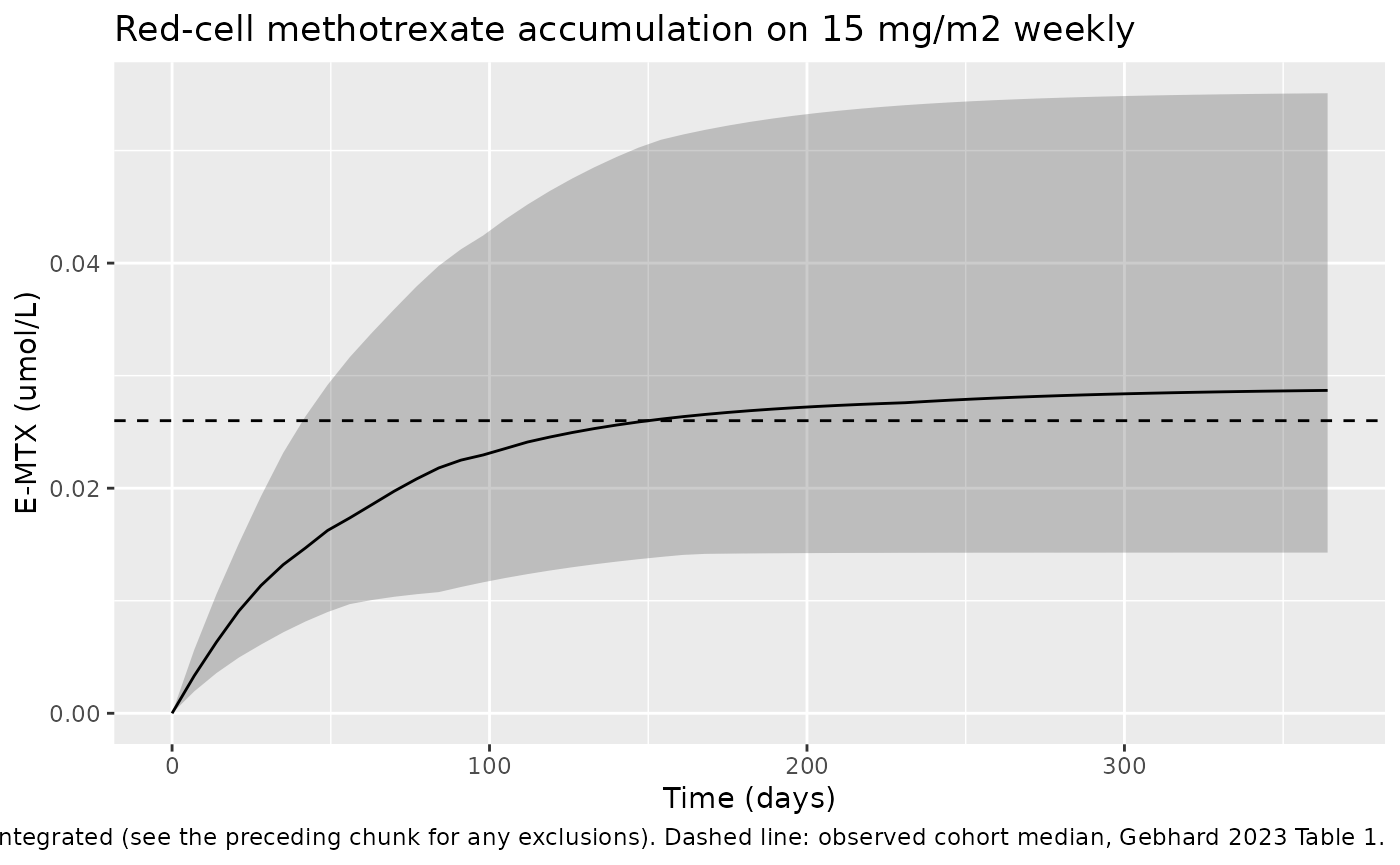
The approach to plateau is slow – the model’s red-cell elimination half-life is 38.5 days, which is the property the paper’s Discussion validates against literature red-cell methotrexate half-lives of 30-40 days.

6-Mercaptopurine arm: plasma NCA and the red-cell steady state

mp_dose <- umol_m2(MP_DOSE_MGM2, MW_6MP)

ka_mp <- exp(mp6[["lka"]]); vc_mp <- exp(mp6[["lvc"]])
cl_mp <- exp(mp6[["lcl"]]); kel_mp <- cl_mp / vc_mp
f_mp  <- exp(mp6[["lfdepot"]])

mp_sd_events <- make_arm(
  n = 2L, dose_umol_m2 = mp_dose, interval_days = 1, n_doses = 1L,
  obs_times = seq(0, 0.6, by = 0.002),
  covariates = list(BL_TGN_RBC = 0),
  label = "6MP 57.1 mg/m2 single dose"
)

mp_sd <- rxode2::rxSolve(
  rxode2::zeroRe(mod_6mp), events = mp_sd_events,
  keep = c("treatment"), useLinCmt = FALSE
) |>
  as.data.frame()
#> ℹ omega/sigma items treated as zero: 'etalvmax_rbc', 'etalkeff_rbc'
#> Warning: multi-subject simulation without without 'omega'

# Closed-form one-compartment first-order-absorption references.
tmax_mp <- log(ka_mp / kel_mp) / (ka_mp - kel_mp)
mp_reference <- tibble::tibble(
  treatment  = "6MP 57.1 mg/m2 single dose",
  cmax       = f_mp * mp_dose / vc_mp * (kel_mp / ka_mp)^(kel_mp / (ka_mp - kel_mp)),
  tmax       = tmax_mp,
  aucinf.obs = f_mp * mp_dose / cl_mp,
  half.life  = log(2) / kel_mp
)
mp_reference
#> # A tibble: 1 × 5
#>   treatment                   cmax   tmax aucinf.obs half.life
#>   <chr>                      <dbl>  <dbl>      <dbl>     <dbl>
#> 1 6MP 57.1 mg/m2 single dose 0.952 0.0553      0.145    0.0450

mp_conc <- mp_sd |>
  dplyr::filter(!is.na(Cc)) |>
  dplyr::select(id, time, Cc, treatment)

mp_conc <- dplyr::bind_rows(
  mp_conc,
  mp_conc |> dplyr::distinct(id, treatment) |>
    dplyr::mutate(time = 0, Cc = 0)
) |>
  dplyr::distinct(id, treatment, time, .keep_all = TRUE) |>
  dplyr::arrange(id, treatment, time)

mp_dose_df <- mp_sd_events |>
  dplyr::filter(evid == 1) |>
  dplyr::select(id, time, amt, treatment)

mp_nca <- PKNCA::pk.nca(PKNCA::PKNCAdata(
  PKNCA::PKNCAconc(mp_conc, Cc ~ time | treatment + id),
  PKNCA::PKNCAdose(mp_dose_df, amt ~ time | treatment + id),
  intervals = data.frame(
    start = 0, end = Inf,
    cmax = TRUE, tmax = TRUE, aucinf.obs = TRUE, half.life = TRUE
  )
))

mp_cmp <- nlmixr2lib::ncaComparisonTable(
  simulated = mp_nca,
  reference = mp_reference,
  by        = "treatment",
  units     = c(cmax = "umol/L", tmax = "day",
                aucinf.obs = "umol*day/L", half.life = "day"),
  tolerance_pct = 20
)
knitr::kable(
  mp_cmp,
  caption = "6-Mercaptopurine plasma NCA against closed-form references. * differs by >20%."
)

6-Mercaptopurine plasma NCA against closed-form references. * differs by >20%.
NCA parameter	treatment	Reference	Simulated	% diff
Cmax (umol/L)	6MP 57.1 mg/m2 single dose	0.952	0.952	-0.0%
Tmax (day)	6MP 57.1 mg/m2 single dose	0.0553	0.056	+1.3%
AUC0-∞ (obs) (umol*day/L)	6MP 57.1 mg/m2 single dose	0.145	0.145	-0.0%
t½ (day)	6MP 57.1 mg/m2 single dose	0.045	0.0467	+3.8%

mp_wide <- as.data.frame(mp_nca) |>
  dplyr::filter(start == 0, is.infinite(end)) |>
  dplyr::group_by(PPTESTCD) |>
  dplyr::summarise(value = mean(PPORRES), .groups = "drop")
get_mp <- function(x) mp_wide$value[match(x, mp_wide$PPTESTCD)]

stopifnot(
  abs(get_mp("aucinf.obs") / mp_reference$aucinf.obs - 1) < 0.02,
  abs(get_mp("cmax")       / mp_reference$cmax       - 1) < 0.02,
  abs(get_mp("half.life")  / mp_reference$half.life  - 1) < 0.05
)

Plasma 6-mercaptopurine turns over very fast – an absorption half-life of 0.79 h and an elimination half-life of 1.08 h – so on daily dosing the plasma concentration is a narrow daily spike, not a sustained level. That matters for the red-cell influx, because the Michaelis-Menten term saturates during the spike: the average influx over a day is well below the value the average plasma concentration would suggest.

mp_ss_events <- make_arm(
  n = N_PER_ARM, dose_umol_m2 = mp_dose, interval_days = 1, n_doses = 180L,
  obs_times = seq(0, 179, by = 3),
  covariates = list(BL_TGN_RBC = 0),
  label = "6MP 57.1 mg/m2 daily"
)
stopifnot(!anyDuplicated(unique(mp_ss_events[, c("id", "time", "evid")])))

mp_ss <- rxode2::rxSolve(
  mod_6mp, events = mp_ss_events, keep = c("treatment"), useLinCmt = FALSE
) |>
  as.data.frame()

vmax_mp <- exp(mp6[["lvmax_rbc"]])
km_mp   <- exp(mp6[["lkm_rbc"]])
keff_mp <- exp(mp6[["lkeff_rbc"]])

cbar_mp    <- f_mp * mp_dose / (cl_mp * 1)
etgn_naive <- vmax_mp * cbar_mp / (km_mp + cbar_mp) / keff_mp

# Typical-value run sampled finely across the final dosing interval, so the
# influx integral can be evaluated. The Michaelis-Menten influx has no closed
# form under a time-varying plasma concentration, so the check here is the
# mass balance itself: at steady state the cycle-average influx must equal the
# cycle-average efflux.
mp_typ_events <- make_arm(
  n = 2L, dose_umol_m2 = mp_dose, interval_days = 1, n_doses = 180L,
  obs_times = sort(unique(c(seq(0, 178, by = 3), seq(178, 179, by = 0.005)))),
  covariates = list(BL_TGN_RBC = 0),
  label = "6MP 57.1 mg/m2 daily (typical)"
)
mp_typ <- rxode2::rxSolve(
  rxode2::zeroRe(mod_6mp), events = mp_typ_events, useLinCmt = FALSE
) |>
  as.data.frame()
#> ℹ omega/sigma items treated as zero: 'etalvmax_rbc', 'etalkeff_rbc'
#> Warning: multi-subject simulation without without 'omega'

mp_cycle    <- mp_typ |> dplyr::filter(id == 1, time >= 178, time <= 179)
mp_influx   <- mean(vmax_mp * mp_cycle$Cc / (km_mp + mp_cycle$Cc))
mp_efflux   <- keff_mp * mean(mp_cycle$rbc_tgn)
etgn_typ    <- mean(mp_cycle$rbc_tgn)
etgn_popmed <- median(mp_ss$rbc_tgn[mp_ss$time >= 120])

tibble::tibble(
  Quantity = c(
    "mean plasma 6MP over a dosing interval (umol/L)",
    "naive plateau V_mm mean(C) / (K_mm + mean(C)) / K_eff (umol/L)",
    "cycle-average red-cell influx, day 178-179 (umol/L/day)",
    "cycle-average red-cell efflux K_eff x mean(E-TGN) (umol/L/day)",
    "simulated typical-value cycle-mean E-TGN (umol/L)",
    "simulated population median E-TGN, day 120-179 (umol/L)",
    "observed cohort median E-TGN (umol/L)"
  ),
  Value = c(cbar_mp, etgn_naive, mp_influx, mp_efflux, etgn_typ,
            etgn_popmed, 0.83),
  Source = c("derived", "derived (upper bound)", "this simulation",
             "this simulation", "this simulation", "this simulation",
             "Gebhard 2023 Table 1")
) |>
  dplyr::mutate(Value = signif(Value, 4)) |>
  knitr::kable(caption = "Red-cell thioguanine-nucleotide steady state (PK-only model, Table 3 parameters).")

Red-cell thioguanine-nucleotide steady state (PK-only model, Table 3 parameters).
Quantity	Value	Source
mean plasma 6MP over a dosing interval (umol/L)	0.14480	derived
naive plateau V_mm mean(C) / (K_mm + mean(C)) / K_eff (umol/L)	2.10800	derived (upper bound)
cycle-average red-cell influx, day 178-179 (umol/L/day)	0.03750	this simulation
cycle-average red-cell efflux K_eff x mean(E-TGN) (umol/L/day)	0.03782	this simulation
simulated typical-value cycle-mean E-TGN (umol/L)	0.92260	this simulation
simulated population median E-TGN, day 120-179 (umol/L)	0.82050	this simulation
observed cohort median E-TGN (umol/L)	0.83000	Gebhard 2023 Table 1


stopifnot(
  # Mass balance at steady state: influx == efflux over a full dosing cycle.
  abs(mp_influx / mp_efflux - 1) < 0.03,
  # Jensen's inequality: the Michaelis-Menten influx is concave in the plasma
  # concentration, so averaging a spiky profile must give strictly LESS than
  # evaluating the function at the average concentration. This is a structural
  # property of the model, so it is asserted rather than described.
  etgn_typ < etgn_naive,
  # And the plateau must land near the cohort's observed median.
  abs(etgn_typ / 0.83 - 1) < 0.25
)

The typical-value plateau of 0.923 umol/L is within 11% of the observed cohort median of 0.83 umol/L (Table 1) – the closest thing this paper offers to an external check on the 6MP red-cell submodel, since no NCA summaries are published. The steady-state mass balance closes to 0.9%, and the Jensen bound holds: the naive plateau computed from the average plasma concentration (2.11 umol/L) over-estimates by more than a factor of two because the saturable influx spends most of the day well below V_mm.

Joint PKPD model

Steady-state hold (no drug)

The Friberg chain’s initial conditions were written by the authors as X_prol(0) = ... = X_tr3(0) = inieff x base x k_ma / k_tr with X_ma(0) = inieff x base, but the symbol k_ma is never defined anywhere in the paper or the supplement. It is nonetheless uniquely determined: the authors state “we assume to have reached a treatment steady state”, and setting dX_ma/dt = k_tr X_tr3 - k_circ X_ma = 0 with X_ma(0) = inieff x base forces X_tr3(0) = inieff x base x k_circ / k_tr, i.e. k_ma == k_circ.

The test below is what makes that derivation checkable rather than asserted. With inieff set to 1 and no drug given, the encoded initial conditions must hold the whole chain exactly at base for all time. Any other reading of k_ma breaks this identity immediately.

mod_hold <- mod_pkpd |>
  rxode2::ini(linieff = 0) |>   # inieff = exp(0) = 1
  rxode2::zeroRe()
#> ℹ change initial estimate of `linieff` to `0`

# The joint model has two endpoints (E-TGN and ANC), so rxode2 requires a
# `dvid` on every observation row to disambiguate the dvid -> cmt mapping.
# Both observables are returned as columns regardless of which endpoint the
# row names, so dvid = 1 is sufficient for a pure simulation.
hold_events <- tibble::tibble(id = 1:2, BL_TGN_RBC = 0) |>
  tidyr::crossing(time = seq(0, 200, by = 1)) |>
  dplyr::mutate(amt = NA_real_, evid = 0L, cmt = "central", dvid = 1L)

hold <- rxode2::rxSolve(mod_hold, events = hold_events, useLinCmt = FALSE) |>
  as.data.frame()
#> ℹ omega/sigma items treated as zero: 'etalvmax_rbc', 'etalkeff_rbc', 'etalrbase', 'etalktr', 'etalslope', 'etalgamma', 'etalinieff'
#> Warning: multi-subject simulation without without 'omega'

base_tv <- exp(mp[["lrbase"]])
max_drift <- max(abs(hold$ANC - base_tv))

c(base = base_tv, max_abs_drift = max_drift, relative = max_drift / base_tv)
#>          base max_abs_drift      relative 
#>  2.170000e+00  1.127779e-07  5.197140e-08

# Exact hold: with no drug and inieff = 1, every state derivative is zero at
# t = 0 and stays zero. Tolerance is integrator noise, not model behaviour.
stopifnot(max_drift / base_tv < 1e-6)

The chain holds at 2.17 G/L with a maximum relative drift of 5.2^{-8} over 200 days. This simultaneously confirms the k_ma == k_circ derivation, the k_prol = k_tr constraint the authors carried from Jost et al., and the (base / X_ma)^gamma feedback normalisation.

Typical-value dose-response

The paper’s own simulations (Figures 3-4, Supplementary Figure S23) are typical-value trajectories, so the dose-response check is run the same way. Monotonicity is a structural consequence of the linear effect function Edrug = slope x E-TGN acting on the proliferation rate, so it is asserted.

DOSE_ARMS <- c(`25 mg/m2/day` = 25, `57.1 mg/m2/day` = 57.1, `100 mg/m2/day` = 100)

make_pkpd_arm <- function(dose_mgm2, label, n, id_offset) {
  make_arm(
    n = n, dose_umol_m2 = umol_m2(dose_mgm2, MW_6MP),
    interval_days = 1, n_doses = 180L, obs_times = seq(0, 179, by = 3),
    covariates = list(BL_TGN_RBC = 0), id_offset = id_offset, label = label
  ) |>
    # Two endpoints -> observation rows need a dvid (see the hold chunk above).
    dplyr::mutate(dvid = ifelse(evid == 0L, 1L, NA_integer_))
}

typ_events <- dplyr::bind_rows(lapply(seq_along(DOSE_ARMS), function(i) {
  make_pkpd_arm(DOSE_ARMS[[i]], names(DOSE_ARMS)[i], n = 2L,
                id_offset = (i - 1L) * 2L)
}))

pkpd_typ <- rxode2::rxSolve(
  rxode2::zeroRe(mod_pkpd), events = typ_events,
  keep = c("treatment"), useLinCmt = FALSE
) |>
  as.data.frame() |>
  dplyr::mutate(
    treatment = factor(as.character(treatment), levels = names(DOSE_ARMS))
  )
#> ℹ omega/sigma items treated as zero: 'etalvmax_rbc', 'etalkeff_rbc', 'etalrbase', 'etalktr', 'etalslope', 'etalgamma', 'etalinieff'
#> Warning: multi-subject simulation without without 'omega'

typ_summary <- pkpd_typ |>
  dplyr::filter(time >= 120) |>
  dplyr::group_by(treatment) |>
  dplyr::summarise(
    `ANC (G/L)`      = median(ANC),
    `E-TGN (umol/L)` = median(rbc_tgn),
    `Edrug`          = median(rbc_tgn) * exp(mp[["lslope"]]),
    .groups = "drop"
  ) |>
  dplyr::rename(`Dose arm` = treatment)

knitr::kable(
  typ_summary, digits = 3,
  caption = "Typical-value plateau (day 120-179) by dose arm. Gebhard 2023 Table 1 reports a cohort median ANC of 1.6 G/L and E-TGN of 0.83 umol/L at a median dose of 57.1 mg/m2/day."
)

Typical-value plateau (day 120-179) by dose arm. Gebhard 2023 Table 1 reports a cohort median ANC of 1.6 G/L and E-TGN of 0.83 umol/L at a median dose of 57.1 mg/m2/day.
Dose arm	ANC (G/L)	E-TGN (umol/L)	Edrug
25 mg/m2/day	1.810	0.702	0.112
57.1 mg/m2/day	1.698	0.966	0.155
100 mg/m2/day	1.621	1.144	0.183

typ_anc  <- typ_summary$`ANC (G/L)`
typ_etgn <- typ_summary$`E-TGN (umol/L)`

stopifnot(
  # Strictly monotone dose-response in both directions.
  all(diff(typ_anc)  < 0),
  all(diff(typ_etgn) > 0),
  # Every arm stays below the drug-free baseline.
  all(typ_anc < base_tv),
  # The published median dose reproduces the cohort medians of Table 1.
  abs(typ_anc[2]  / 1.6  - 1) < 0.20,
  abs(typ_etgn[2] / 0.83 - 1) < 0.25
)

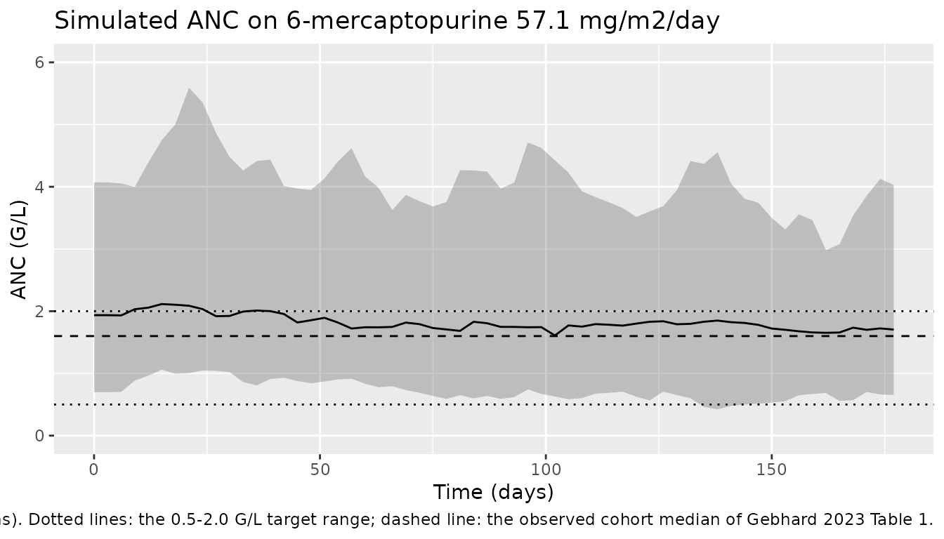
At the published median dose of 57.1 mg/m^2/day the typical-value plateau is 1.7 G/L for ANC and 0.966 umol/L for E-TGN, against the cohort medians of 1.6 G/L and 0.83 umol/L in Table 1. Both land within a quarter of the published values with no fitting whatsoever – every parameter is transcribed – which is the strongest external check the paper supports, since it reports no NCA or exposure summaries.

Population variability at the published median dose

pkpd_events <- make_pkpd_arm(MP_DOSE_MGM2, "57.1 mg/m2/day", n = N_PER_ARM,
                             id_offset = 0L)
stopifnot(!anyDuplicated(unique(pkpd_events[, c("id", "time", "evid")])))

pkpd_all <- rxode2::rxSolve(
  mod_pkpd, events = pkpd_events, keep = c("treatment"), useLinCmt = FALSE
) |>
  as.data.frame()

# A handful of subjects in the upper tail of the V_mm / K_eff variability push
# E-TGN past the ceiling where Edrug = slope x E-TGN exceeds 1; the
# proliferation term k_tr X_prol (1 - Edrug) fb then turns negative, the
# circulating pool collapses toward zero, the (base / X_ma)^gamma feedback
# diverges, and the solver returns NA. That is a property of the published
# linear effect function (see "Range of validity" below), not of the encoding.
# Those subjects are excluded from the percentile summary and the exclusion is
# reported explicitly -- a silent NA would bias every percentile below.
failed_ids <- unique(pkpd_all$id[is.na(pkpd_all$ANC)])
pkpd <- pkpd_all |> dplyr::filter(!(id %in% failed_ids))

c(subjects_simulated = N_PER_ARM,
  subjects_diverged  = length(failed_ids),
  fraction_diverged  = length(failed_ids) / N_PER_ARM)
#> subjects_simulated  subjects_diverged  fraction_diverged 
#>              1e+02              1e+00              1e-02

# The summary is only meaningful if divergence is a tail phenomenon.
stopifnot(length(failed_ids) / N_PER_ARM < 0.05, !anyNA(pkpd$ANC))

pkpd |>
  dplyr::group_by(time) |>
  dplyr::summarise(
    Q05 = quantile(ANC, 0.05), Q50 = median(ANC),
    Q95 = quantile(ANC, 0.95), .groups = "drop"
  ) |>
  ggplot(aes(time, Q50)) +
  geom_ribbon(aes(ymin = Q05, ymax = Q95), alpha = 0.25) +
  geom_line() +
  geom_hline(yintercept = c(0.5, 2.0), linetype = "dotted") +
  geom_hline(yintercept = 1.6, linetype = "dashed") +
  coord_cartesian(ylim = c(0, 6)) +
  labs(
    x = "Time (days)", y = "ANC (G/L)",
    title = "Simulated ANC on 6-mercaptopurine 57.1 mg/m2/day",
    caption = paste(
      "Median and 5th-95th percentile of the virtual subjects that",
      "integrated (see the preceding chunk for any exclusions).",
      "Dotted lines: the 0.5-2.0 G/L target range; dashed line: the",
      "observed cohort median of Gebhard 2023 Table 1."
    )
  )

pop_late <- pkpd |> dplyr::filter(time >= 120)
pop_med_anc  <- median(pop_late$ANC)
pop_med_etgn <- median(pop_late$rbc_tgn)

tibble::tibble(
  Quantity = c(
    "median ANC, day 120-179 (G/L)",
    "observed cohort median ANC (G/L)",
    "median E-TGN, day 120-179 (umol/L)",
    "observed cohort median E-TGN (umol/L)",
    "fraction of ANC observations inside 0.5-2.0 G/L"
  ),
  Value = c(pop_med_anc, 1.6, pop_med_etgn, 0.83,
            mean(pop_late$ANC >= 0.5 & pop_late$ANC <= 2.0)),
  Source = c("this simulation", "Gebhard 2023 Table 1", "this simulation",
             "Gebhard 2023 Table 1", "this simulation")
) |>
  dplyr::mutate(Value = signif(Value, 4)) |>
  knitr::kable(caption = "Population summary at the published median dose.")

Population summary at the published median dose.
Quantity	Value	Source
median ANC, day 120-179 (G/L)	1.7460	this simulation
observed cohort median ANC (G/L)	1.6000	Gebhard 2023 Table 1
median E-TGN, day 120-179 (umol/L)	0.8162	this simulation
observed cohort median E-TGN (umol/L)	0.8300	Gebhard 2023 Table 1
fraction of ANC observations inside 0.5-2.0 G/L	0.5808	this simulation


stopifnot(
  abs(pop_med_anc  / 1.6  - 1) < 0.25,
  abs(pop_med_etgn / 0.83 - 1) < 0.25
)

Range of validity of the linear effect function

Edrug = slope x E-TGN with slope = 0.16 L/umol reaches 1 once E-TGN passes 1 / 0.16 = 6.25 umol/L, at which point the proliferation term k_tr X_prol (1 - Edrug) fb turns negative. The observed E-TGN range in Table 1 runs to 7.6 umol/L, so the published model is used right at – and past – that limit inside its own data set. This is a property of the published linear effect function, not of the encoding, and it is reported here rather than hidden by trimming the cohort.

etgn_ceiling <- 1 / exp(mp[["lslope"]])

tibble::tibble(
  Quantity = c(
    "E-TGN ceiling where Edrug = 1 (umol/L)",
    "typical-value E-TGN at the highest simulated dose (umol/L)",
    "maximum E-TGN over the surviving population arm (umol/L)",
    "subjects that diverged, of 100 simulated",
    "fraction of surviving population observations with Edrug > 1",
    "observed maximum E-TGN, Table 1 (umol/L)"
  ),
  Value = c(
    etgn_ceiling,
    max(pkpd_typ$rbc_tgn),
    max(pkpd$rbc_tgn),
    length(failed_ids),
    mean(pkpd$rbc_tgn > etgn_ceiling),
    7.6
  ),
  Source = c("derived", "this simulation", "this simulation",
             "this simulation", "this simulation", "Gebhard 2023 Table 1")
) |>
  dplyr::mutate(Value = signif(Value, 4)) |>
  knitr::kable(caption = "Where the linear effect function stops being interpretable.")

Where the linear effect function stops being interpretable.
Quantity	Value	Source
E-TGN ceiling where Edrug = 1 (umol/L)	6.250	derived
typical-value E-TGN at the highest simulated dose (umol/L)	1.144	this simulation
maximum E-TGN over the surviving population arm (umol/L)	2.847	this simulation
subjects that diverged, of 100 simulated	1.000	this simulation
fraction of surviving population observations with Edrug > 1	0.000	this simulation
observed maximum E-TGN, Table 1 (umol/L)	7.600	Gebhard 2023 Table 1


# Typical-value trajectories -- the ones the paper itself simulates -- stay
# comfortably inside the interpretable range across the whole dose span.
stopifnot(max(pkpd_typ$rbc_tgn) < etgn_ceiling)

At the published median dose the effect function is comfortably inside its interpretable range: every surviving trajectory peaks at less than half the ceiling, and no surviving observation has Edrug > 1. The exception is the tail – the 1 subject(s) that diverged, drawn from the upper tail of the V_mm / K_eff variability, are exactly the ones whose E-TGN ran past 6.25 umol/L. Since Table 1’s own observed E-TGN range reaches 7.6 umol/L, real patients in this cohort sat above the ceiling too. Users simulating above the published dose range should check this bound explicitly; it is a property of the published linear effect function, not of the encoding.

Assumptions and deviations

Residual errors are read as variances, not standard deviations. Gebhard 2023 never states which. The 6MP arm decides it: read as variances, the combined residual SD at the cohort median E-TGN of 0.83 umol/L is sqrt(0.023 + (0.253 x 0.83)^2) = 0.259 umol/L, matching the observed median / mean individual-prediction RMSE of 0.21 / 0.24 (Table 3); read as standard deviations it would be 0.058, about 3.6x too small. The ANC reading corroborates this independently: as a variance, 0.25 gives a 50% proportional CV, so at the estimated baseline of 2.17 G/L the residual SD is 1.09 G/L against Table 4’s population-prediction median / mean ANC RMSE of 1.12 / 1.27 G/L. The implied CVs are also the only plausible ones for monthly red-cell metabolite assays (15.5% for E-MTX, 25.3% for E-TGN, 50% for ANC, versus 2.4% / 6.4% / 25% under the standard-deviation reading). All three model files encode sqrt(...) inline so the reading is visible.
k_ma is derived, not transcribed. The symbol appears in the published initial conditions but is defined nowhere in the paper or supplement. It is uniquely determined as k_ma == k_circ = 2.3765 1/day by the authors’ own “treatment steady state” assumption; the steady-state hold test above is the check that this is the intended reading.
The plasma micro-constants are reparameterised. Supplementary Tables S1, S2 and S11 report ka, ke, k_cp, k_pc, V_C, V_P; the model files carry the canonical lka / lcl / lvc / lq / lvp. The mapping is exact and is verified above against the paper’s own printed k_pc = 2.64 and its stated derivation of V_P.
Dose units are derived. The paper never states the units of the plasma concentrations; they are pinned to umol/L by dimensional analysis of equations MTX4c and 6MP3b (see “Units and dosing convention”). Doses must therefore be supplied in umol/m^2. The mg-to-umol conversion factors (methotrexate 454.44 g/mol, 6-mercaptopurine 152.18 g/mol) are standard molecular weights, not values printed in the paper.
The final PKPD model carries no methotrexate arm. Table 5 does report K_in^MTX, K_eff^MTX and MTX residual errors, because the MTX arm was carried during estimation to fit the E-MTX observations. It never enters the effect function, so it cannot influence ANC – consistent with Supplementary section I, which lists no MTX states, and with the Discussion’s “our final PKPD model does not include a MTX PK submodel”. That arm is packaged separately as Gebhard_2023_methotrexate, so no published endpoint is lost. Note that the MTX rate constants estimated jointly (0.032 / 0.019, Table 5) differ trivially from the standalone MTX fit (0.031 / 0.018, Table 2); the standalone model file carries the Table 2 values, which are the estimates of the model it represents.
The 6MP red-cell parameters differ between the two 6MP files. The standalone PK model carries Table 3 (V_mm 0.096, K_mm 0.016, K_eff 0.041) and the joint PKPD model carries Table 5 (V_mm 0.21, K_mm 0.14, K_eff 0.050). This is the paper’s own finding – “for the 6MP PK submodel, both V_mm and K_mm increase distinctly” when the ANC data are fitted jointly – not a transcription discrepancy. The two files are not interchangeable.
Red-cell compartments are started at zero in this vignette. The published models initialise them at the patient’s first observed concentration (covariates BL_MTX_RBC / BL_TGN_RBC), because every record begins mid-therapy. Starting from zero with a long run-in is used here so the simulated steady states are produced by the model’s own kinetics rather than imported from data; Gebhard 2023’s Discussion names exactly this timeline restructuring as the preferable alternative. Users reproducing individual patient trajectories should supply the observed baselines instead.
The virtual cohort is dosed at fixed published medians. In the real study, doses were titrated per patient against the white-blood-cell count, which is a feedback loop the model does not contain. Fixed-dose arms are therefore an idealisation, and the cohort medians in Table 1 – which mix dose levels, titration history, and incompletely accumulated red-cell pools – are an approximate rather than an exact comparator.
No covariate model. Gebhard 2023 reports no covariate effects on any parameter; volumes and clearances are expressed per m^2 so body-surface area cancels, and no allometric or maturation terms appear. The only per-subject inputs are the red-cell baselines and (for methotrexate) the dose level feeding the saturable bioavailability term.
No erratum or corrigendum was found for doi:10.1038/s41598-023-38414-0.