Gentamicin and tobramycin with radiomic biological age (Alikhani 2025)
Source:vignettes/articles/Alikhani_2025_gentamicin_tobramycin.Rmd
Alikhani_2025_gentamicin_tobramycin.RmdModel and source
- Citation: Alikhani R, Horbal SR, Pai MP. A comparison between radiomic biological age and chronological age in estimating kidney function. Sci Rep. 2025;15:13384. doi:10.1038/s41598-025-98297-1.
- Article: https://doi.org/10.1038/s41598-025-98297-1 (open access, with Supplementary Material 1 holding Supplementary Tables 1-5)
Alikhani, Horbal and Pai used aminoglycoside clearance as a surrogate for kidney function and asked whether “radiomic biological age” indices built from abdominal CT body-composition measurements (analytic morphomics) explain clearance better than chronological age. The structural model is a one-compartment model with zero-order (infusion) input and linear elimination, fitted in Monolix to pooled gentamicin and tobramycin concentrations. Each age index is divided by serum creatinine and enters CL as a power term; drug (tobramycin vs gentamicin) enters V.
The paper reports four complete final models side by side (Supplementary Table 4), one per age index. All four are packaged:
| Model file | Paper model | Age index on CL | AIC |
|---|---|---|---|
Alikhani_2025_gentamicin_tobramycin_bamor1 |
19.1 | BAMor_1 = psoas muscle area x BMD / fascia area | 2601.57 |
Alikhani_2025_gentamicin_tobramycin_bamor2 |
25.1 | BAMor_2 = psoas muscle area x psoas muscle density x vertebral slab height | 2601.71 |
Alikhani_2025_gentamicin_tobramycin_bamor3 |
29.2 | BAMor_3 = dorsal muscle group area x BMD / visceral fat area, plus subcutaneous fat density | 2598.33 (best) |
Alikhani_2025_gentamicin_tobramycin_ca |
6.1 | 1 / chronological age | 2602.12 |
AIC values are from Table 3 and Supplementary Table 3.
Population
156 hospitalised adults at the University of Michigan Health System
who received at least three doses of gentamicin (n = 67) or tobramycin
(n = 89, 57.05%) with measured plasma concentrations and had an
abdominal CT scan (Alikhani 2025 Table 1). 51.92% were female; median
age 58 years (IQR 22, range 21-93); mean weight 81.0 kg (SD 21.06, range
43.8-139.3); median serum creatinine 0.75 mg/dL (IQR 0.57, range
0.17-5.5). Psoas measures were taken at L4, the dorsal muscle group at
L2 and the remaining morphomics at L3; missing morphomic values were
imputed (random-forest mice). Dosing regimens were not
reported.
The same information is available programmatically via
readModelDb("Alikhani_2025_gentamicin_tobramycin_bamor3")()$population.
Source trace
Every ini() value carries an in-file comment pointing at
its source. All structural, covariate, IIV and residual-error values
come from Supplementary Table 4 (one column per model). Monolix reports
the random effects as SDs (Omega_V, Omega_Cl);
the model files hold their squares.
| Parameter | BAMor_1 (19.1) | BAMor_2 (25.1) | BAMor_3 (29.2) | CA (6.1) | Source |
|---|---|---|---|---|---|
lcl (Cl_pop, L/h) |
log(5.8) | log(5.72) | log(2.62) | log(5.82) | Supp Table 4 |
lvc (V_pop gentamicin, L) |
log(49.09) | log(45.87) | log(45.89) | log(49.2) | Supp Table 4 |
| index exponent on CL | 0.15 | 0.12 | 0.11 | 0.19 | Supp Table 4 ‘Beta_Cl_(BAMor/creat)’, ‘Beta_Cl_(CA-1/creat)’ |
e_ct_subcutaneous_fat_density_cl |
– | – | -0.93 | – | Supp Table 4 ‘Beta_Cl_(subcutfathu)’ |
e_trt_tobramycin_vc |
0.24 | 0.29 | 0.28 | 0.25 | Supp Table 4 ‘Beta_V_drug_tobramycin’ |
etalcl (variance) |
0.49^2 | 0.51^2 | 0.49^2 | 0.49^2 | Supp Table 4 ‘Omega_Cl’ |
etalvc (variance) |
0.37^2 | 0.37^2 | 0.36^2 | 0.38^2 | Supp Table 4 ‘Omega_V’ |
addSd (a, mg/L) |
0.049 | 0.12 | 0.13 | 0.069 | Supp Table 4 ‘a’ |
propSd (b) |
0.4 | 0.38 | 0.39 | 0.4 | Supp Table 4 ‘b’ |
| Equation | Source |
|---|---|
| One compartment, infusion input, linear CL, log-normal IIV on V and CL | Results; Methods |
Combined error y = f + sqrt(a^2 + (b f)^2) e
(“combined2”) |
Supp Table 3 row 4 (base model) |
V = V_pop exp(beta TRT_TOBRAMYCIN + eta_V) |
Supp Table 4 ‘V_drug_Gentamicin’ / ‘V_drug_Tobramycin’ |
| BAMor_1, BAMor_2, BAMor_3 definitions | Table 2 |
CL = Cl_pop (BAMor_1 / Scr / 10)^beta |
Supp Table 3 rows 19 / 19.1 |
CL = Cl_pop (BAMor_2 / Scr / 4200000)^beta |
Supp Table 3 rows 25 / 25.1 |
CL = Cl_pop (BAMor_3 / (Scr x 300))^beta exp(beta_subQ SubQHU / 90) |
Equation 1 (centring constant 300; see Assumptions) |
CL = Cl_pop ((1 / (Age x Scr)) / 0.03)^beta |
Supp Table 3 rows 6 / 6.1 |
Deterministic checks
Tobramycin volume
Supplementary Table 4 also prints the volume for each drug category.
Applying the drug effect to V_pop must reproduce the
tobramycin row; the residual difference comes from the 2-decimal
rounding of the published coefficient (an exponent rounded by 0.005
moves V by up to 0.5%).
model_names <- c(
  BAMor_1 = "Alikhani_2025_gentamicin_tobramycin_bamor1",
  BAMor_2 = "Alikhani_2025_gentamicin_tobramycin_bamor2",
  BAMor_3 = "Alikhani_2025_gentamicin_tobramycin_bamor3",
  CA = "Alikhani_2025_gentamicin_tobramycin_ca"
)
mods <- lapply(model_names, function(nm) rxode2::rxode(readModelDb(nm)))
#> ℹ parameter labels from comments will be replaced by 'label()'
#> ℹ parameter labels from comments will be replaced by 'label()'
#> ℹ parameter labels from comments will be replaced by 'label()'
#> ℹ parameter labels from comments will be replaced by 'label()'

theta_of <- function(m) {
  df <- m$iniDf
  stats::setNames(df$est[is.na(df$neta1)], df$name[is.na(df$neta1)])
}
thetas <- lapply(mods, theta_of)

# Typical-value (zeroRe) solves are intended throughout; muffle only the
# notices rxode2 gives for them, so any other warning still surfaces.
solve_typical <- function(mod, events, ...) {
  withCallingHandlers(
    rxode2::rxSolve(rxode2::zeroRe(mod), events = events, ...),
    warning = function(w) {
      if (grepl("without 'omega'", conditionMessage(w), fixed = TRUE)) {
        invokeRestart("muffleWarning")
      }
    },
    message = function(m) {
      if (grepl("treated as zero", conditionMessage(m), fixed = TRUE)) {
        invokeRestart("muffleMessage")
      }
    }
  )
}

v_check <- tibble(
  model = names(model_names),
  v_gent = vapply(thetas, function(t) exp(t[["lvc"]]), numeric(1)),
  v_tobra = vapply(thetas, function(t) exp(t[["lvc"]] + t[["e_trt_tobramycin_vc"]]), numeric(1)),
  v_tobra_published = c(62.38, 61.61, 60.75, 63.42) # Supp Table 4 'V_drug_Tobramycin'
) |>
  mutate(pct_diff = 100 * (v_tobra / v_tobra_published - 1))
stopifnot(nrow(v_check) == 4L, all(abs(v_check$pct_diff) < 1))

v_check |>
  dplyr::rename(
    "Model" = model,
    "V gentamicin (L)" = v_gent,
    "V tobramycin, model (L)" = v_tobra,
    "V tobramycin, Supp Table 4 (L)" = v_tobra_published,
    "Difference (%)" = pct_diff
  ) |>
knitr::kable(digits = 2, caption = "Volume of distribution by drug.")| Model | V gentamicin (L) | V tobramycin, model (L) | V tobramycin, Supp Table 4 (L) | Difference (%) |
|---|---|---|---|---|
| BAMor_1 | 49.09 | 62.41 | 62.38 | 0.04 |
| BAMor_2 | 45.87 | 61.30 | 61.61 | -0.50 |
| BAMor_3 | 45.89 | 60.72 | 60.75 | -0.05 |
| CA | 49.20 | 63.17 | 63.42 | -0.39 |
Typical clearance at the cohort centre
The paper notes that the BAMor_3 model’s Cl_pop (2.62
L/h) is far below the other three (5.72-5.82 L/h). That is a property of
where each index is centred, not a disagreement between models:
Cl_pop is the clearance when the index term equals one, and
for BAMor_3 that point is far from a typical patient (and its
subcutaneous-fat term is uncentred). Evaluating all four models at the
cohort’s Table 1 centre (mean morphomics, median age and serum
creatinine) puts them within a few percent of each other.
centre <- data.frame(
  id = 1L,
  AGE = 58, # Table 1 median
  CREAT = 0.75, # Table 1 median, mg/dL
  CT_PSOAS_MUSCLE_AREA = 1953.7 / 100, # Table 1 mean, mm^2 -> cm^2
  CT_PSOAS_MUSCLE_DENSITY = 46.28, # HU
  CT_DORSAL_MUSCLE_AREA = 4030 / 100, # mm^2 -> cm^2
  CT_FASCIA_AREA = 50625 / 100, # mm^2 -> cm^2
  VISCERAL_ABDOMINAL_FAT = 12790 / 100, # mm^2 -> cm^2
  CT_SUBCUTANEOUS_FAT_DENSITY = -89.03, # HU
  CT_VERTEBRAL_BMD = 182.23, # HU
  CT_VERTEBRAL_SLAB_HEIGHT = 32.78, # mm
  TRT_TOBRAMYCIN = 0L
)
ev_centre <- rxode2::et(amt = 100, cmt = "central") |>
  rxode2::et(time = 1, cmt = "central") |>
  as.data.frame() |>
  mutate(id = 1L) |>
  left_join(centre, by = "id")

cl_centre <- vapply(mods, function(m) {
  solve_typical(m, events = ev_centre)$cl[1]
}, numeric(1))

# Hand-computed from the published equations at the same covariates.
cl_hand <- c(
  BAMor_1 = 5.8 * ((1953.7 * 182.23 / 50625) / 0.75 / 10)^0.15,
  BAMor_2 = 5.72 * (1953.7 * 46.28 * 32.78 / 0.75 / 4200000)^0.12,
  BAMor_3 = 2.62 * ((4030 * 182.23 / 12790) / (0.75 * 300))^0.11 * exp(-0.93 * -89.03 / 90),
  CA = 5.82 * ((1 / (58 * 0.75)) / 0.03)^0.19
)
stopifnot(max(abs(cl_centre / cl_hand[names(cl_centre)] - 1)) < 1e-8)
# Four independently fitted models of the same data should agree on the
# typical patient; a mis-transcribed exponent or centring constant moves one of
# them by tens of percent.
stopifnot(max(cl_centre) / min(cl_centre) < 1.10)

# Serum creatinine divides every index, so doubling it must scale CL by
# exactly 2^-beta in each model; this pins where CREAT enters the equation.
ev_centre_2scr <- ev_centre |> mutate(CREAT = 2 * CREAT)
cl_2scr <- vapply(mods, function(m) {
  solve_typical(m, events = ev_centre_2scr)$cl[1]
}, numeric(1))
beta_scr <- c(
  BAMor_1 = 0.15, BAMor_2 = 0.12, BAMor_3 = 0.11, CA = 0.19 # Supp Table 4
)
stopifnot(max(abs(cl_2scr / cl_centre - 2^-beta_scr[names(cl_centre)])) < 1e-8)

tibble(
  model = names(cl_centre),
  cl_pop = vapply(thetas, function(t) exp(t[["lcl"]]), numeric(1)),
  cl_centre = cl_centre
) |>
  dplyr::rename(
    "Model" = model,
    "Cl_pop, Supp Table 4 (L/h)" = cl_pop,
    "Typical CL at cohort centre (L/h)" = cl_centre
  ) |>
knitr::kable(digits = 2, caption = "Population CL versus typical CL at the Table 1 centre.")| Model | Cl_pop, Supp Table 4 (L/h) | Typical CL at cohort centre (L/h) |
|---|---|---|
| BAMor_1 | 5.80 | 5.74 |
| BAMor_2 | 5.72 | 5.68 |
| BAMor_3 | 2.62 | 5.66 |
| CA | 5.82 | 5.53 |
Closed-form one-compartment infusion
A typical-value solve of the BAMor_3 model for a 30-minute infusion is compared against the analytic one-compartment infusion solution.
dose <- 400
tinf <- 0.5
ev_cf <- data.frame(
  id = 1L,
  time = c(0, seq(0.1, 24, by = 0.1)),
  evid = c(1L, rep(0L, 240)),
  amt = c(dose, rep(0, 240)),
  rate = c(dose / tinf, rep(0, 240)),
  cmt = "central"
) |>
  left_join(centre, by = "id")
sim_cf <- solve_typical(mods$BAMor_3,
  events = ev_cf,
  rtol = 1e-10, atol = 1e-12
) |>
  as.data.frame()
k <- sim_cf$cl[1] / sim_cf$vc[1]
analytic <- with(sim_cf, ifelse(
  time <= tinf,
  dose / tinf / cl * (1 - exp(-k * time)),
  dose / tinf / cl * (1 - exp(-k * tinf)) * exp(-k * (time - tinf))
))
rel_err <- max(abs(sim_cf$Cc / analytic - 1))
stopifnot(rel_err < 1e-6)
rel_err
#> [1] 1.001782e-10
Virtual cohort
Individual data are not public. The cohort below draws each covariate independently from the Table 1 summaries (normal for symmetric measures, log-normal for serum creatinine and visceral fat area, which Table 1 shows as right-skewed), truncated to the published ranges. Correlations between the morphomic measures are not reported and are not reproduced.
The dosing regimen was not reported. The simulation uses an illustrative 5 mg/kg (actual body weight) dose infused over 30 minutes every 24 hours for three doses (the inclusion criterion was at least three doses).
rxode2::rxSetSeed(20250418)
set.seed(20250418)

rtnorm <- function(n, mean, sd, lo, hi) {
  x <- stats::rnorm(n, mean, sd)
  bad <- x < lo | x > hi
  while (any(bad)) {
    x[bad] <- stats::rnorm(sum(bad), mean, sd)
    bad <- x < lo | x > hi
  }
  x
}
rtlnorm <- function(n, meanlog, sdlog, lo, hi) {
  exp(rtnorm(n, meanlog, sdlog, log(lo), log(hi)))
}

n_per_drug <- 150L
vat_sdlog <- sqrt(log(1 + (10708.68 / 12790)^2)) # mean/SD-matched log-normal
make_cohort <- function(n, tobra, id_offset) {
  tibble(
    id = id_offset + seq_len(n),
    drug = if (tobra == 1L) "Tobramycin" else "Gentamicin",
    TRT_TOBRAMYCIN = tobra,
    WT = rtnorm(n, 81.0, 21.06, 43.8, 139.3),
    AGE = rtnorm(n, 58, 22 / 1.349, 21, 93),
    # Median 0.75, IQR 0.57: log-normal sdlog solves 0.75*2*sinh(0.674 s) = 0.57
    CREAT = rtlnorm(n, log(0.75), asinh(0.57 / 1.5) / 0.674, 0.17, 5.5),
    CT_PSOAS_MUSCLE_AREA = rtnorm(n, 1953.7, 748.63, 455.5, 4353.5) / 100,
    CT_PSOAS_MUSCLE_DENSITY = rtnorm(n, 46.28, 11.73, 0.24, 72.64),
    CT_DORSAL_MUSCLE_AREA = rtnorm(n, 4030, 1123.49, 1024, 7950) / 100,
    CT_FASCIA_AREA = rtnorm(n, 50625, 14102.61, 26787, 112550) / 100,
    VISCERAL_ABDOMINAL_FAT = rtlnorm(
      n, log(12790) - vat_sdlog^2 / 2, vat_sdlog, 40, 49471
    ) / 100,
    CT_SUBCUTANEOUS_FAT_DENSITY = rtnorm(n, -89.03, 12.76, -112.08, -59.83),
    CT_VERTEBRAL_BMD = rtnorm(n, 182.23, 63.03, 46.35, 588.30),
    CT_VERTEBRAL_SLAB_HEIGHT = rtnorm(n, 32.78, 3.83, 20.46, 42.13)
  )
}
cohort <- bind_rows(
  make_cohort(n_per_drug, 0L, 0L),
  make_cohort(n_per_drug, 1L, n_per_drug)
)
stopifnot(!anyDuplicated(cohort$id))

tau <- 24
dose_times <- c(0, 24, 48)
obs_times <- sort(unique(c(seq(0, 48, by = 2), seq(48, 72, by = 0.25))))
events <- bind_rows(
  cohort |>
    tidyr::crossing(time = dose_times) |>
    mutate(evid = 1L, amt = 5 * WT, rate = amt / 0.5),
  cohort |>
    tidyr::crossing(time = obs_times) |>
    mutate(evid = 0L, amt = 0, rate = 0)
) |>
  mutate(cmt = "central") |>
  arrange(id, time, desc(evid))
Simulation
sims <- bind_rows(lapply(names(mods), function(nm) {
  rxode2::rxSolve(mods[[nm]],
    events = events,
    keep = c("drug", "WT")
  ) |>
    as.data.frame() |>
    mutate(model = nm)
}))
Replicate published figures
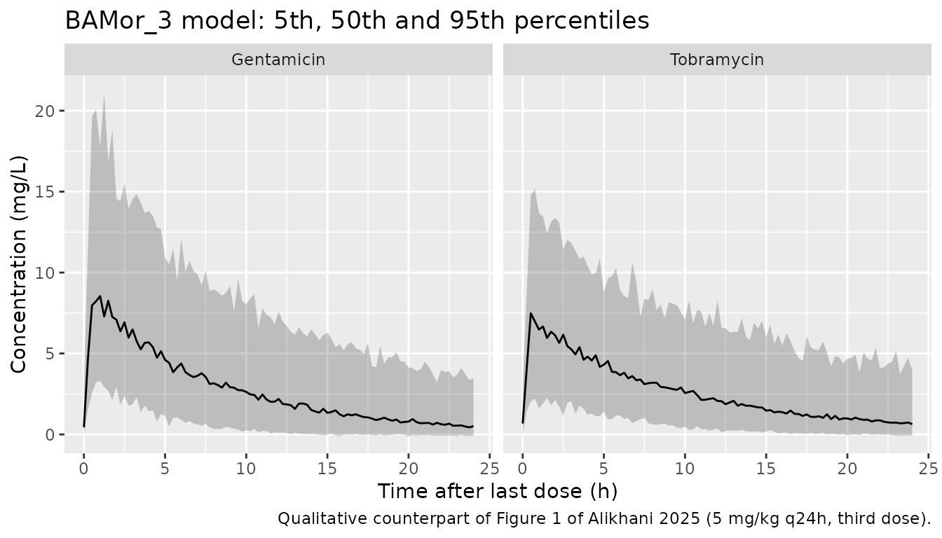
Figure 1: concentration versus time after last dose
Figure 1 of the paper is a VPC of the BAMor_3 model, stratified by drug, with time after last dose on the x-axis. The observed regimens are unknown, so the panel below is a qualitative counterpart under the illustrative regimen above (the third dose, 48-72 h), not an overlay. The features that do not depend on dose carry over: a near-mono-exponential decline over the dosing interval and lower concentrations for tobramycin at the same mg/kg dose, from its roughly 1.3-fold larger V.
sims |>
  filter(model == "BAMor_3", time >= 48) |>
  mutate(tad = time - 48) |>
  group_by(drug, tad) |>
  summarise(
    Q05 = quantile(sim, 0.05, na.rm = TRUE),
    Q50 = quantile(sim, 0.50, na.rm = TRUE),
    Q95 = quantile(sim, 0.95, na.rm = TRUE),
    .groups = "drop"
  ) |>
  ggplot(aes(tad, Q50)) +
  geom_ribbon(aes(ymin = Q05, ymax = Q95), alpha = 0.25) +
  geom_line() +
  facet_wrap(~drug) +
  labs(
    x = "Time after last dose (h)", y = "Concentration (mg/L)",
    title = "BAMor_3 model: 5th, 50th and 95th percentiles",
    caption = "Qualitative counterpart of Figure 1 of Alikhani 2025 (5 mg/kg q24h, third dose)."
  )
Clearance across the four age indices
Individual typical clearances (no random effects) of the same virtual subjects under each model. The exponents on the indices are small (0.11-0.19), so serum creatinine moves typical CL only modestly, and in the BAMor_3 model the subcutaneous fat density term (log-CL SD about 0.93 x 12.76 / 90 = 0.13 across the cohort) outweighs the creatinine term (about 0.11 x 0.55 = 0.06). Because the virtual covariates are drawn independently, the agreement between models below is lower than it would be in the real cohort, where the morphomic measures, age and creatinine are correlated; the table is descriptive.
cl_typ <- bind_rows(lapply(names(mods), function(nm) {
  solve_typical(mods[[nm]],
    events = events |> filter(evid == 1L | time == 72),
    keep = "drug"
  ) |>
    as.data.frame() |>
    distinct(id, .keep_all = TRUE) |>
    transmute(id, drug, cl, model = nm)
}))
cl_wide <- cl_typ |>
  tidyr::pivot_wider(names_from = model, values_from = cl)
cl_cor <- stats::cor(log(cl_wide[, names(mods)]))
stopifnot(nrow(cl_wide) == 2L * n_per_drug, !anyNA(cl_cor))
knitr::kable(cl_cor, digits = 2, caption = "Correlation of log typical CL between models (virtual cohort).")| BAMor_1 | BAMor_2 | BAMor_3 | CA | |
|---|---|---|---|---|
| BAMor_1 | 1.00 | 0.76 | 0.39 | 0.61 |
| BAMor_2 | 0.76 | 1.00 | 0.27 | 0.67 |
| BAMor_3 | 0.39 | 0.27 | 1.00 | 0.31 |
| CA | 0.61 | 0.67 | 0.31 | 1.00 |
cl_typ |>
  left_join(cohort |> select(id, CREAT), by = "id") |>
  ggplot(aes(CREAT, cl)) +
  geom_point(alpha = 0.3, size = 0.8) +
  facet_wrap(~model, nrow = 1) +
  scale_x_log10() +
  scale_y_log10() +
  labs(x = "Serum creatinine (mg/dL)", y = "Typical CL (L/h)")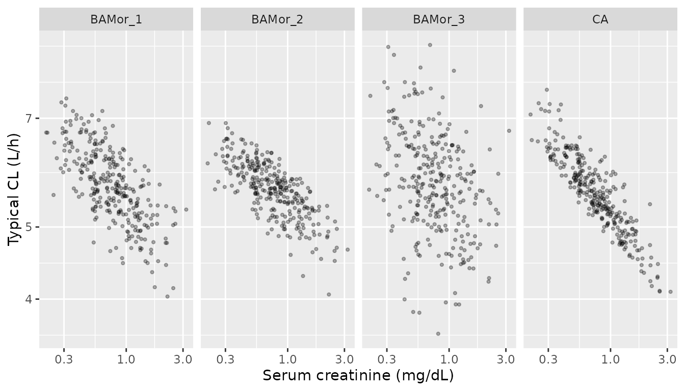
PKNCA validation
AUC over the third dosing interval (48-72 h) from PKNCA is compared
with the closed form for the same subject,
Dose / CL x (1 - exp(-3 k tau)) (exact for a linear
one-compartment model after three equal doses). Both sides use the same
drawn parameters, so the difference is numerical (integrator plus
trapezoid on the 0.25 h grid) and a tight bound is appropriate.
sim_nca <- sims |>
  filter(!is.na(Cc), time >= 48) |>
  select(id, time, Cc, drug, model)

conc_obj <- PKNCA::PKNCAconc(sim_nca, Cc ~ time | model + drug + id)
dose_df <- events |>
  filter(evid == 1L, time == 48) |>
  select(id, time, amt, drug) |>
  tidyr::crossing(model = names(mods))
dose_obj <- PKNCA::PKNCAdose(dose_df, amt ~ time | model + drug + id)
intervals <- data.frame(start = 48, end = 72, cmax = TRUE, auclast = TRUE)
nca_res <- PKNCA::pk.nca(PKNCA::PKNCAdata(conc_obj, dose_obj, intervals = intervals))

auc_nca <- as.data.frame(nca_res) |>
  filter(PPTESTCD == "auclast") |>
  select(id, model, drug, auclast = PPORRES)
auc_cf <- sims |>
  filter(time == 72) |>
  transmute(id, model, auc_cf = 5 * WT / cl * (1 - exp(-3 * cl / vc * tau)))
chk <- inner_join(auc_nca, auc_cf, by = c("id", "model")) |>
  mutate(pct_diff = 100 * (auclast / auc_cf - 1))
stopifnot(nrow(chk) == 4L * 2L * n_per_drug)
stopifnot(abs(median(chk$pct_diff)) < 0.5, max(abs(chk$pct_diff)) < 2)

chk |>
  group_by(model, drug) |>
  summarise(
    n = n(),
    auc_median = median(auclast),
    auc_cf_median = median(auc_cf),
    max_abs_pct = max(abs(pct_diff)),
    .groups = "drop"
  ) |>
  dplyr::rename(
    "Model" = model,
    "Drug" = drug,
    "N" = n,
    "Median PKNCA AUC48-72 (mg*h/L)" = auc_median,
    "Median closed-form AUC (mg*h/L)" = auc_cf_median,
    "Max abs difference (%)" = max_abs_pct
  ) |>
knitr::kable(digits = 2, caption = "PKNCA AUC over the third dosing interval versus the closed form.")| Model | Drug | N | Median PKNCA AUC48-72 (mg*h/L) | Median closed-form AUC (mg*h/L) | Max abs difference (%) |
|---|---|---|---|---|---|
| BAMor_1 | Gentamicin | 150 | 68.03 | 68.05 | 0.21 |
| BAMor_1 | Tobramycin | 150 | 71.60 | 71.61 | 0.18 |
| BAMor_2 | Gentamicin | 150 | 65.93 | 65.94 | 0.55 |
| BAMor_2 | Tobramycin | 150 | 73.21 | 73.21 | 0.24 |
| BAMor_3 | Gentamicin | 150 | 70.01 | 70.02 | 0.16 |
| BAMor_3 | Tobramycin | 150 | 68.73 | 68.74 | 0.12 |
| CA | Gentamicin | 150 | 66.76 | 66.77 | 0.17 |
| CA | Tobramycin | 150 | 74.78 | 74.81 | 0.20 |
The paper reports no NCA results, so there is no published NCA table to compare against.
Assumptions and deviations
-
BAMor_3 centring constant. The printed final-model
Equation 1 divides BAMor_3 by
Scr x 300; the modelling log (Supplementary Table 3, rows 29, 29.1 and 29.2) writes the same index with/580. Equation 1 is otherwise inconsistent with model 29.2: its coefficients 0.12 and -0.92 are those of the age-only model 32.1 (Supplementary Table 5), not 29.2’s 0.11 and -0.93; its intercept 0.42 equals log10(2.62) rather than ln(2.62); and it addsexp(eta_Cl)on the log scale whereeta_Clis meant. The maintainers kept 300 from the printed equation and the coefficients from Supplementary Table 4. With 580 the typical CL at the cohort centre would be (300/580)^0.11 = 0.93 times the value above (about 5.3 instead of 5.7 L/h). -
Concentration units. The paper gives CL in L/h and
V in L but does not state the concentration units; mg/L (dose in mg) is
assumed, the clinical convention for aminoglycosides, which makes the
additive error
amg/L. - CT area units. The new CT area covariates are supplied in cm^2 (the convention of the existing visceral-fat covariate); the source reports mm^2. BAMor_1 and BAMor_3 use ratios of two areas, so the conversion cancels; BAMor_2 multiplies the psoas area by 100 inside the model to reach the mm^2 scale on which its centring constant (4200000) was set.
- Subcutaneous fat density units. Table 1 labels it mm2; it is a CT attenuation in HU (Supplementary Table 2), which its values (-112 to -60) confirm.
- Age-only models not packaged. Supplementary Table 5 refits each index without serum creatinine and drug; the paper treats these as a reduced sensitivity analysis (two of them were “incomplete in Monolix”), so only the four complete final models of Supplementary Table 4 are packaged.
- Missing standard error. Supplementary Table 4 gives no SE for the BAMor_3 index exponent (0.11, RSE 29.4%); the value is used as printed.
- Virtual cohort. Covariates are drawn independently from Table 1 marginal summaries; the real morphomic measures are correlated with one another and with age and sex, so the spread of the indices is only approximate. The dosing regimen (5 mg/kg q24h, 30-minute infusion) is illustrative.
- Errata. No correction notice is linked to the article (PMID 40251375) in Europe PMC’s comment-and-correction records as of 2026-11-10.