Darbepoetin alfa in chemotherapy-induced anemia (Agoram 2006) • nlmixr2lib

Model and source

Agoram 2006 develops two models, fitted sequentially, and nlmixr2lib ships them as two files so that each is usable on its own:

Model	Role	Source table
`Agoram_2006_darbepoetin_alfa_cia`	Population PK of darbepoetin alfa in chemotherapy-induced anemia (CIA), freely estimated with its full random-effects structure	Table 3
`Agoram_2006_darbepoetin_alfa_cia_hemoglobin`	PK/PD model of the hemoglobin response, with the PK layer held at the Table 3 fixed effects	Table 4

The paper is explicit that the second stage reuses the first: “the Pk model consisted of fixed-effects parameters obtained from the full covariate model; random IIV and RRV in the Pk model were ignored”. The PD file therefore wraps every PK entry in fixed() and carries no PK etas – that is the model the authors actually fitted, not a simplification introduced here.

Citation: Agoram B, Heatherington AC, Gastonguay MR. Development and evaluation of a population pharmacokinetic-pharmacodynamic model of darbepoetin alfa in patients with nonmyeloid malignancies undergoing multicycle chemotherapy. The AAPS Journal. 2006;8(3):E552-E563. doi:10.1208/aapsj080364
Article: https://doi.org/10.1208/aapsj080364
PubMed Central: https://www.ncbi.nlm.nih.gov/pmc/articles/PMC2761062/

mod_pk <- readModelDb("Agoram_2006_darbepoetin_alfa_cia")
mod_pd <- readModelDb("Agoram_2006_darbepoetin_alfa_cia_hemoglobin")

ui_pk <- rxode2::rxode(mod_pk)
#> ℹ parameter labels from comments will be replaced by 'label()'
ui_pd <- rxode2::rxode(mod_pd)
#> ℹ parameter labels from comments will be replaced by 'label()'

PK model – Two-compartment population PK model with first-order subcutaneous absorption for darbepoetin alfa in adults with nonmyeloid malignancies and chemotherapy-induced anemia (Agoram 2006, AAPS J). Both IV and SC routes are supported. Body weight modifies clearance and central volume via a normalized power model (reference 70 kg), and receiving more than two cycles of platinum-containing chemotherapy during the PK assessment multiplies clearance by 0.737. Total measured serum concentration is the sum of the simulated darbepoetin alfa and an individual-specific endogenous-erythropoietin (eEPO) constant that the ELISA assay cross-detects. Exponential (log-normal) residual error. This is the PK layer of the paper’s sequentially fitted PK/PD analysis; the hemoglobin response model is Agoram_2006_darbepoetin_alfa_cia_hemoglobin.

PK/PD model – Sequentially fitted PK/PD model of the hemoglobin response to darbepoetin alfa in adults with nonmyeloid malignancies and chemotherapy-induced anemia (Agoram 2006, AAPS J). The two-compartment PK layer is carried at the fixed-effect estimates of the full covariate PK model (Agoram_2006_darbepoetin_alfa_cia) with its interindividual and residual variability deliberately dropped, exactly as the paper fitted the PD stage. Serum darbepoetin alfa concentration stimulates a zero-order hemoglobin production rate through an Emax-type term (incremental Smax = 43.7%, S50 = 3.68 ng/mL), feeding a Friberg-style catenary chain: one progenitor transit compartment of mean transit time RBCPT = 4.68 days followed by four equal-transit-time mature red-cell lifespan compartments summing to RBCLS = 82.2 days. Total hemoglobin is the sum of the four lifespan compartments. Receiving any concomitant platinum-containing chemotherapy multiplies S50 by 1.86. Additive residual error on hemoglobin.

Note that a different Agoram 2006 paper is also in the library: Agoram_2006_darbepoetin_alfa is the healthy-subject popPK model from Br J Clin Pharmacol 63(1):41-52. Same first author, same year, same drug, different study population – hence the _cia suffix here.

Population

The PK model was built on 140 patients and 1442 serum darbepoetin alfa concentrations pooled from two Amgen studies (990146, n = 56, IV or SC 2.25 ug/kg QW; 20010162, n = 84, SC 6.75 ug/kg Q3W). The PK/PD model was built on a larger, partly disjoint set of 573 patients and 6356 hemoglobin observations from studies 20010162, 980290 and 980291, spanning SC doses from 0.5 ug/kg QW to 15 ug/kg Q3W. Hemoglobin data from study 990146 were excluded from the PD analysis because its hemoglobin entry criterion differed substantially from the other studies (Agoram 2006 Table 1).

Patients were adults (>= 18 years) with nonmyeloid malignancies receiving cyclic chemotherapy, anemic as a result of cancer or chemotherapy, with ECOG performance status 0-2 and adequate renal and hepatic function. Baseline characteristics (Agoram 2006 Table 2) for the combined PK/PD set: 70% female, age mean 60.1 years (SD 12.3, range 20-91), body weight mean 69.9 kg (SD 16.2, range 39-136), baseline hemoglobin mean 9.96 g/dL (SD 1.00, range 5.5-12.3). Tumor types were breast 31%, lung 17%, gastrointestinal 17%, gynecologic 17%, genitourinary 7%, lymphoma 2%, other 9%. Race was screened as a covariate but is not tabulated in the publication.

The same information is available programmatically from either model’s population metadata:

str(ui_pd$population, max.level = 1, give.attr = FALSE)
#> List of 14
#>  $ species       : chr "human"
#>  $ n_subjects    : int 573
#>  $ n_studies     : int 3
#>  $ n_observations: int 6356
#>  $ age_range     : chr "20-91 years (combined PkPd data set; Agoram 2006 Table 2)"
#>  $ age_median    : chr "Mean 60.1 years, SD 12.3 (median not tabulated)"
#>  $ weight_range  : chr "39-136 kg (combined PkPd data set; Agoram 2006 Table 2)"
#>  $ weight_median : chr "Mean 69.9 kg, SD 16.2 (median not tabulated)"
#>  $ sex_female_pct: num 70
#>  $ race_ethnicity: chr "Screened as a PD covariate but not tabulated in Agoram 2006."
#>  $ disease_state : chr "Adults (>= 18 years) with nonmyeloid malignancies receiving cyclic chemotherapy, with chemotherapy-induced anem"| __truncated__
#>  $ dose_range    : chr "0.5 to 4.5 ug/kg SC QW, 3.0 to 9.0 ug/kg SC Q2W, 4.5 to 15 ug/kg SC Q3W and 9.0 to 18.0 ug/kg SC Q4W across stu"| __truncated__
#>  $ regions       : chr "Three Amgen-sponsored clinical studies (20010162, 980290, 980291); geographic sites not stated in the publication."
#>  $ notes         : chr "PkPd model development data set: 573 patients and 6356 hemoglobin observations pooled from Amgen studies 200101"| __truncated__

Source trace

Every ini() entry in both model files carries an in-file comment naming the table it came from. They are collected here for review.

Structure

Equation / structure	Source location
Two-compartment disposition, first-order SC absorption, bioavailability `F`	Figure 1A; Results, “Pharmacokinetic Model”
Total measured serum concentration = darbepoetin alfa + endogenous EPO (assay cross-reactivity)	Analytical Methods; Equation 2
Log-normal IIV, `P_i = TVP * exp(eta)`	Equation 1
Log-transformed exponential (log-normal) PK residual error	Equation 2
Normalized power / categorical covariate model	Equation 3
`TVCL = theta_CL * theta_1^X * (BWT/70)^theta_2`, `X = 1` if PCNT > 2	Equation 12
`TVV1 = theta_V1 * (BWT/70)^theta_3`	Equation 13
Indirect response, `dHb/dt = Rin - Kout * Hb`, `Hb(0) = Hb0`, `0 = Rin - Kout * Hb0`	Equations 4, 5, 6
`dA1/dt = Rin * Stim - kPT * A1` (progenitor compartment)	Equation 7
`Stim = 1 + Smax * C_DA / (S50 + C_DA)`	Equation 8
`dA2/dt = kPT * A1 - kLS * A2`; `dAi/dt = kLS * A(i-1) - kLS * Ai`, `i = 3,4,5`	Equations 9, 10
`Hb = sum(Ai, i = 2..5)`	Equation 11
`kPT = 1 / RBCPT`, `kLS = 4 / RBCLS`	Text following Equation 6
`TVS50 = theta_S50 * theta_4^X`, `X = 1` if PCNT > 0	Equation 14

Parameters

Parameter	Model file entry	Value	Source
CL	`lcl`	2010 mL/day	Table 3
V1	`lvc`	3390 mL	Table 3
V2	`lvp`	251 mL	Table 3
Q	`lq`	2900 mL/day	Table 3
Ka	`lka`	0.318 /day	Table 3
F	`lfdepot`	0.443	Table 3
C0 (eEPO)	`leepo`	0.415 ng/mL	Table 3
theta_1 (PCNT on CL)	`e_conmed_platin_gt2_cl`	0.737	Table 3
theta_2 (BWT on CL)	`e_wt_cl`	0.623	Table 3
theta_3 (BWT on V1)	`e_wt_vc`	0.639	Table 3
omega^2 CL, CL-V1, V1	`etalcl + etalvc` block	0.181, 0.134, 0.225	Table 3
omega^2 Ka	`etalka`	0.0883	Table 3
omega^2 C0	`etaleepo`	0.501	Table 3
sigma_1^2	`expSd`	0.483 (SD = 0.695)	Table 3
RBCPT	`lmtt`	4.68 day	Table 4
RBCLS	`lmtt_rbc`	82.2 day	Table 4
Smax	`lemax`	0.437	Table 4
S50	`lec50`	3.68 ng/mL	Table 4
Hb0	`lrbase_hb`	9.92 g/dL	Table 4
theta_4 (PCNT on S50)	`e_conmed_platin_ec50`	1.86	Table 4
omega^2 RBCLS	`etalmtt_rbc`	1.63	Table 4
omega^2 S50, S50-Hb0, Hb0	`etalec50 + etalrbase_hb` block	8.05, 0.0539, 0.00720	Table 4
sigma_2^2	`addSd_hb`	0.401 (SD = 0.633 g/dL)	Table 4

Part 1 – Pharmacokinetics

Replicating Figure 2C

Figure 2C of Agoram 2006 overlays the mean model prediction on observed mean concentrations after a single 2.25 ug/kg IV dose, a single 2.25 ug/kg SC dose, and a single 6.75 ug/kg SC dose, over 21 days. The panel is a typical-value prediction, so between-subject variability is zeroed.

REF_WT <- 70                      # reference / typical weight, Agoram 2006 Eq 12-13

pk_arms <- tibble::tribble(
  ~arm,               ~dose_ug_kg, ~cmt,
  "2.25 ug/kg (IV)",  2.25,        "central",
  "2.25 ug/kg (SC)",  2.25,        "depot",
  "6.75 ug/kg (SC)",  6.75,        "depot"
)

# Dense early grid so Tmax and the alpha phase are resolved; 21 days matches
# the x-range of the published panel and keeps every concentration comfortably
# above solver round-off.
pk_times <- sort(unique(c(
  seq(0, 0.5, by = 0.005), seq(0.5, 3, by = 0.02),
  seq(3, 21, by = 0.1)
)))

make_pk_arm <- function(arm, dose_ug_kg, cmt, id) {
  dplyr::bind_rows(
    tibble(id = id, time = 0, amt = dose_ug_kg * REF_WT, evid = 1L, cmt = cmt),
    # Observation rows point at the ODE state `central`, never at the
    # algebraic observable `Cc`.
    tibble(id = id, time = pk_times, amt = NA_real_, evid = 0L, cmt = "central")
  ) |>
    dplyr::mutate(arm = arm, WT = REF_WT, CONMED_PLATIN_GT2 = 0)
}

pk_events <- dplyr::bind_rows(
  lapply(seq_len(nrow(pk_arms)), function(i) {
    make_pk_arm(pk_arms$arm[i], pk_arms$dose_ug_kg[i], pk_arms$cmt[i], id = i)
  })
)
stopifnot(!anyDuplicated(unique(pk_events[, c("id", "time", "evid")])))

pk_typical <- rxode2::zeroRe(mod_pk)
#> ℹ parameter labels from comments will be replaced by 'label()'
sim_pk <- rxode2::rxSolve(
  pk_typical, events = pk_events, keep = c("arm", "WT"),
  omega = NA, sigma = NA, returnType = "data.frame"
)

# The ELISA cross-detects endogenous erythropoietin, so `Cc` is the TOTAL
# measured concentration (drug + eEPO). The drug-only profile is what the
# structural PK parameters describe, and it is what NCA must be run on -- an
# additive eEPO baseline that never decays would make AUCinf infinite.
sim_pk <- sim_pk |>
  dplyr::filter(!is.na(Cc)) |>
  dplyr::mutate(Cdrug = pmax(Cc - eepo, 0))

ggplot(sim_pk, aes(time, Cc, colour = arm, linetype = arm)) +
  geom_line(linewidth = 0.7) +
  scale_y_log10(limits = c(0.1, 100)) +
  scale_x_continuous(breaks = seq(0, 22, by = 2)) +
  labs(
    x = "Time (days)", y = "Serum concentration (ng/mL)",
    colour = NULL, linetype = NULL,
    title = "Figure 2C -- typical-value profiles after a single dose",
    caption = "Replicates Figure 2C of Agoram 2006 (mean predicted profiles)."
  ) +
  theme_bw() + theme(legend.position = "top")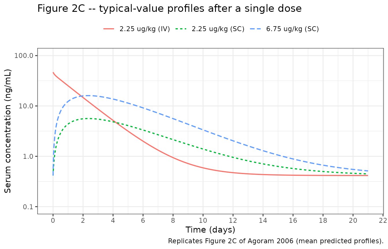

The published panel can be read off at a handful of landmarks. Digitised values below are approximate (gridline resolution of a log-scale figure), so they are checked with a tolerance rather than asserted exactly.

landmark <- function(arm_name, t) {
  d <- sim_pk[sim_pk$arm == arm_name, ]
  d$Cc[which.min(abs(d$time - t))]
}

fig2c <- tibble::tibble(
  arm = c("2.25 ug/kg (IV)", "2.25 ug/kg (SC)", "6.75 ug/kg (SC)",
          "6.75 ug/kg (SC)", "6.75 ug/kg (SC)"),
  quantity = c("C at 5 min", "Cmax", "Cmax", "C at day 7", "C at day 21"),
  digitised = c(46, 6, 16, 7, 0.55),
  simulated = c(
    landmark("2.25 ug/kg (IV)", 5 / 1440),
    max(sim_pk$Cc[sim_pk$arm == "2.25 ug/kg (SC)"]),
    max(sim_pk$Cc[sim_pk$arm == "6.75 ug/kg (SC)"]),
    landmark("6.75 ug/kg (SC)", 7),
    landmark("6.75 ug/kg (SC)", 21)
  )
)

fig2c |>
  dplyr::mutate(pct_diff = 100 * (simulated - digitised) / digitised) |>
  dplyr::rename(
    "Arm" = arm, "Landmark" = quantity,
    "Digitised from Figure 2C (ng/mL)" = digitised,
    "Simulated (ng/mL)" = simulated,
    "Difference (%)" = pct_diff
  ) |>
  knitr::kable(digits = 2, caption = "Figure 2C landmarks, digitised vs simulated.")

Figure 2C landmarks, digitised vs simulated.
Arm	Landmark	Digitised from Figure 2C (ng/mL)	Simulated (ng/mL)	Difference (%)
2.25 ug/kg (IV)	C at 5 min	46.00	46.55	1.19
2.25 ug/kg (SC)	Cmax	6.00	5.63	-6.24
6.75 ug/kg (SC)	Cmax	16.00	16.05	0.29
6.75 ug/kg (SC)	C at day 7	7.00	7.21	2.97
6.75 ug/kg (SC)	C at day 21	0.55	0.51	-6.76

chk <- 100 * abs(fig2c$simulated - fig2c$digitised) / fig2c$digitised
# Deterministic (typical-value) solve, so this bound does not depend on a
# simulated cohort. 25% is the resolution of reading a 3-decade log axis; a
# mis-transcribed volume, clearance or bioavailability moves these landmarks
# by a factor, not by a quarter.
stopifnot(max(chk) < 25)

PKNCA validation

NCA is run on the baseline-corrected (drug-only) profile of the typical-value solve. Running it over a full-IIV cohort would be misleading here: the half-life estimate is lambda_z-selected per subject and returns NA for subjects whose terminal phase is poorly resolved.

sim_nca <- sim_pk |>
  dplyr::filter(!is.na(Cdrug)) |>
  dplyr::select(id, time, arm, Cc = Cdrug)

# Guarantee a time = 0 record per (id, arm). For the SC arms the pre-dose
# drug concentration is genuinely 0; for the IV arm the t = 0 record already
# exists at the post-dose value and `distinct()` keeps it.
sim_nca <- dplyr::bind_rows(
  sim_nca,
  sim_nca |> dplyr::distinct(id, arm) |> dplyr::mutate(time = 0, Cc = 0)
) |>
  dplyr::distinct(id, arm, time, .keep_all = TRUE) |>
  dplyr::arrange(id, arm, time)

conc_obj <- PKNCA::PKNCAconc(as.data.frame(sim_nca), Cc ~ time | arm + id)

dose_df <- pk_events |>
  dplyr::filter(evid == 1L) |>
  dplyr::select(id, time, amt, arm)
dose_obj <- PKNCA::PKNCAdose(as.data.frame(dose_df), amt ~ time | arm + id)

intervals <- data.frame(
  start = 0, end = Inf,
  cmax = TRUE, tmax = TRUE, auclast = TRUE, aucinf.obs = TRUE,
  half.life = TRUE, aucpext.obs = TRUE
)

nca_res <- PKNCA::pk.nca(PKNCA::PKNCAdata(conc_obj, dose_obj, intervals = intervals))

nca_wide <- as.data.frame(nca_res) |>
  dplyr::select(arm, PPTESTCD, PPORRES) |>
  tidyr::pivot_wider(names_from = PPTESTCD, values_from = PPORRES)

nca_wide |>
  dplyr::select(arm, cmax, tmax, auclast, aucinf.obs, half.life, aucpext.obs) |>
  dplyr::rename(
    "Arm" = arm,
    "Cmax (ng/mL)" = cmax,
    "Tmax (day)" = tmax,
    "AUC0-21d (ng*day/mL)" = auclast,
    "AUC0-inf (ng*day/mL)" = aucinf.obs,
    "t1/2 (day)" = half.life,
    "AUC extrapolated (%)" = aucpext.obs
  ) |>
  knitr::kable(digits = 3, caption = "PKNCA summary of the typical-value single-dose profiles.")

PKNCA summary of the typical-value single-dose profiles.
Arm	Cmax (ng/mL)	Tmax (day)	AUC0-21d (ng*day/mL)	AUC0-inf (ng*day/mL)	t1/2 (day)	AUC extrapolated (%)
2.25 ug/kg (IV)	46.460	0.00	78.358	78.358	1.259	0.001
2.25 ug/kg (SC)	5.210	2.36	34.609	34.714	2.240	0.303
6.75 ug/kg (SC)	15.631	2.36	103.827	104.143	2.240	0.303

Agoram 2006 reports no NCA table of its own – it notes only that the model parameters “generally agreed with previously reported noncompartmental values”. The NCA output is therefore checked against two identities that the structural model must satisfy exactly. These are deterministic consequences of a typical-value solve, not cohort statistics, so they are asserted tightly.

get_nca <- function(arm_name, param) {
  v <- nca_wide[[param]][nca_wide$arm == arm_name]
  if (length(v) != 1L) stop("no unique NCA row for arm '", arm_name, "' / ", param)
  v
}

cl_typ    <- 2.010                              # L/day, Table 3, at WT = 70 kg, PCNT <= 2
dose_iv   <- 2.25 * REF_WT                      # ug
auc_iv    <- get_nca("2.25 ug/kg (IV)", "aucinf.obs")
auc_sc225 <- get_nca("2.25 ug/kg (SC)", "aucinf.obs")

identities <- tibble::tibble(
  Identity = c(
    "AUC0-inf (IV) = Dose / CL",
    "AUC0-inf (SC) / AUC0-inf (IV) = F"
  ),
  Expected = c(dose_iv / cl_typ, 0.443),
  Observed = c(auc_iv, auc_sc225 / auc_iv)
) |>
  dplyr::mutate(`Difference (%)` = 100 * (Observed - Expected) / Expected)

knitr::kable(identities, digits = 4, caption = "Closed-form identities the NCA output must satisfy.")

Closed-form identities the NCA output must satisfy.
Identity	Expected	Observed	Difference (%)
AUC0-inf (IV) = Dose / CL	78.3582	78.3583	0.0001
AUC0-inf (SC) / AUC0-inf (IV) = F	0.4430	0.4430	0.0048


# Both sides come from the same deterministic solve, so the only error is
# numerical (trapezoidal AUC plus lambda_z extrapolation). 1.5% has ample
# headroom over that and still fails on a transcribed CL or F.
stopifnot(max(abs(identities$`Difference (%)`)) < 1.5)
# Terminal extrapolation must be small enough that AUC0-inf is meaningful.
stopifnot(max(nca_wide$aucpext.obs) < 1)

Both SC arms carry a terminal half-life longer than the IV arm (2.24 vs 1.26 days), which is the flip-flop behaviour Agoram 2006 attributes to absorption rate-limited kinetics: Ka (0.318 /day) is smaller than the disposition beta, so the SC terminal slope is the absorption rate constant.

Part 2 – Hemoglobin response

Baseline is a true steady state

The paper writes the indirect-response baseline as 0 = Rin - Kout * Hb0 (Equation 6) but implements the response as a transit chain, so Rin has to be recovered from the chain’s own drug-free steady state. With kPT = 1/RBCPT and kLS = 4/RBCLS, that state is A1 = Rin/kPT and A2 = ... = A5 = Rin/kLS, giving Hb0 = 4*Rin/kLS = Rin*RBCLS, hence Rin = Hb0/RBCLS. If that derivation were wrong the model would drift away from its own baseline with no drug on board – which is exactly what this check tests.

ss_events <- tibble(
  id = 1L, time = seq(0, 365, by = 7), amt = NA_real_, evid = 0L, cmt = "central",
  WT = REF_WT, CONMED_PLATIN = 0, CONMED_PLATIN_GT2 = 0
)

pd_typical <- rxode2::zeroRe(mod_pd)
#> ℹ parameter labels from comments will be replaced by 'label()'
ss <- rxode2::rxSolve(
  pd_typical, events = ss_events, omega = NA, sigma = NA, returnType = "data.frame"
) |>
  dplyr::filter(!is.na(hb))

stopifnot(nrow(ss) == length(unique(ss_events$time)))
ss_drift <- max(abs(ss$hb - 9.92))
cat(sprintf("Max drift from Hb0 = 9.92 g/dL over one year, drug-free: %.3g g/dL\n", ss_drift))
#> Max drift from Hb0 = 9.92 g/dL over one year, drug-free: 1.24e-14 g/dL
# Deterministic; the only error is solver tolerance.
stopifnot(ss_drift < 1e-6)

Replicating Figure 4 – external predictive check

Figure 4 shows the 2.5th-97.5th percentile band of predicted hemoglobin over 16 weeks in the 302-patient test set, whose “population characteristics and administered doses [were] similar to those used in the modeling data set”. The regimens below are the three represented in the PD development set (Agoram 2006 Table 1). The band is a predictive check, so it is taken from the residual-error-carrying sim column rather than the individual prediction.

# set.seed() seeds R's RNG, not rxode2's. rxode2 partitions its streams per
# solver thread, so this cohort is NOT reproducible across machines with
# different thread counts. Every assertion below is written to hold for any
# cohort the model can produce (see known-vignette-failure-patterns.md #12).
set.seed(20060901)
rxode2::rxSetSeed(20060901)

N_PER_ARM <- 150L                 # cap is 200 per arm
WEEKS     <- 16

pd_arms <- tibble::tribble(
  ~regimen,            ~dose_ug_kg, ~ii_days,
  "2.25 ug/kg QW",     2.25,        7,
  "4.5 ug/kg Q3W",     4.5,         21,
  "6.75 ug/kg Q3W",    6.75,        21
)

make_pd_arm <- function(regimen, dose_ug_kg, ii_days, id_offset) {
  # Body weight from the PD cohort: mean 69.9, SD 16.2, truncated to the
  # observed 39-136 kg range (Agoram 2006 Table 2).
  wt <- pmin(pmax(rnorm(N_PER_ARM, 69.9, 16.2), 39), 136)
  # 61% of the pooled cohort had a platinum-containing regimen; the paper does
  # not tabulate PCNT, so this split is an assumption (see Assumptions below).
  platin <- rbinom(N_PER_ARM, 1, 0.61)
  subj <- tibble(
    id = id_offset + seq_len(N_PER_ARM),
    WT = wt,
    CONMED_PLATIN = platin,
    # PCNT > 2 requires PCNT > 0; over a 16-week window a platinum patient on
    # a 3-weekly cycle receives more than two cycles, so the two indicators
    # coincide here. The mutual-consistency constraint is asserted below.
    CONMED_PLATIN_GT2 = platin,
    regimen = regimen
  )
  dose_times <- seq(0, WEEKS * 7 - 1, by = ii_days)
  doses <- subj |>
    tidyr::crossing(time = dose_times) |>
    dplyr::mutate(amt = dose_ug_kg * WT, evid = 1L, cmt = "depot")
  obs <- subj |>
    tidyr::crossing(time = seq(0, WEEKS * 7, by = 7)) |>
    dplyr::mutate(amt = NA_real_, evid = 0L, cmt = "central")
  dplyr::bind_rows(doses, obs) |> dplyr::arrange(id, time, dplyr::desc(evid))
}

pd_events <- dplyr::bind_rows(
  make_pd_arm(pd_arms$regimen[1], pd_arms$dose_ug_kg[1], pd_arms$ii_days[1],   0L),
  make_pd_arm(pd_arms$regimen[2], pd_arms$dose_ug_kg[2], pd_arms$ii_days[2], 200L),
  make_pd_arm(pd_arms$regimen[3], pd_arms$dose_ug_kg[3], pd_arms$ii_days[3], 400L)
)
stopifnot(!anyDuplicated(unique(pd_events[, c("id", "time", "evid")])))
# Register constraint: CONMED_PLATIN_GT2 = 1 must imply CONMED_PLATIN = 1.
stopifnot(all(pd_events$CONMED_PLATIN_GT2 <= pd_events$CONMED_PLATIN))

sim_pd <- rxode2::rxSolve(
  mod_pd, events = pd_events, keep = c("regimen", "WT", "CONMED_PLATIN"),
  returnType = "data.frame"
) |>
  dplyr::filter(!is.na(hb))
#> ℹ parameter labels from comments will be replaced by 'label()'

stopifnot(nrow(sim_pd) > 0, dplyr::n_distinct(sim_pd$id) == 3L * N_PER_ARM)

band <- sim_pd |>
  dplyr::mutate(week = time / 7) |>
  dplyr::group_by(week) |>
  dplyr::summarise(
    lo  = quantile(sim, 0.025, na.rm = TRUE),
    med = quantile(sim, 0.500, na.rm = TRUE),
    hi  = quantile(sim, 0.975, na.rm = TRUE),
    .groups = "drop"
  )

ggplot(band, aes(week, med)) +
  geom_ribbon(aes(ymin = lo, ymax = hi), fill = "orange", alpha = 0.45) +
  geom_line(linewidth = 0.8) +
  scale_x_continuous(breaks = seq(0, 16, by = 5)) +
  coord_cartesian(ylim = c(5, 17)) +
  labs(
    x = "Time (weeks)", y = "Hemoglobin (g/dL)",
    title = "Figure 4 -- predicted hemoglobin, 2.5th-97.5th percentile band",
    caption = "Replicates Figure 4 of Agoram 2006 (predictive check band, pooled over regimens)."
  ) +
  theme_bw()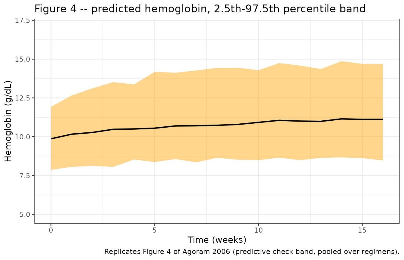

wk <- function(w, col) band[[col]][which.min(abs(band$week - w))]

fig4 <- tibble::tibble(
  Quantity = c(
    "Median Hb at week 0 (g/dL)",
    "Median Hb at week 16 (g/dL)",
    "Rise in median Hb, week 0 to 16 (g/dL)",
    "Lower 2.5th percentile at week 16 (g/dL)",
    "Upper 97.5th percentile at week 16 (g/dL)"
  ),
  `Figure 4 (read off)` = c("~10", "~11.5-12", "~1.5-2", "~8.5", "~13.5-15"),
  Simulated = c(wk(0, "med"), wk(16, "med"), wk(16, "med") - wk(0, "med"),
                wk(16, "lo"), wk(16, "hi"))
)
knitr::kable(fig4, digits = 2, caption = "Figure 4 band, published vs simulated.")

Figure 4 band, published vs simulated.
Quantity	Figure 4 (read off)	Simulated
Median Hb at week 0 (g/dL)	~10	9.87
Median Hb at week 16 (g/dL)	~11.5-12	11.12
Rise in median Hb, week 0 to 16 (g/dL)	~1.5-2	1.25
Lower 2.5th percentile at week 16 (g/dL)	~8.5	8.47
Upper 97.5th percentile at week 16 (g/dL)	~13.5-15	14.68


# Cohort-derived, so these are magnitude bounds with headroom, not tight
# equalities. Week-0 median is anchored by Hb0 = 9.92 with a small IIV
# (omega^2 = 0.0072, ~8.5% CV) plus a 0.633 g/dL residual, so it is the
# stablest of the five.
#
# Realised at 1 / 2 / 4 / 8 solver threads (rxode2 partitions its RNG
# streams per thread, so a 2-core CI runner draws a different cohort than a
# workstation -- see known-vignette-failure-patterns.md #12):
#   med week 0  9.868 - 10.005
#   rise        1.187 -  1.250
#   med week 16 11.074 - 11.193
#   2.5th pct   8.473 -  8.709
#   97.5th pct  14.575 - 15.122
# Every bound below sits outside that range with at least ~0.5 g/dL of
# headroom, and each still goes red on a mis-transcribed Hb0, Smax, S50 or
# RBCLS, which move these numbers by whole g/dL. Do not tighten them back to
# whatever a single local run happens to give.
stopifnot(
  abs(wk(0, "med") - 9.92) < 0.5,
  wk(16, "med") - wk(0, "med") > 0.5,
  wk(16, "med") > 10.5, wk(16, "med") < 12.5,
  wk(16, "lo")  > 7.0,  wk(16, "lo")  < 10.0,
  wk(16, "hi")  > 12.0, wk(16, "hi")  < 17.0
)

The simulated band reproduces the published one in position and in shape: a median that starts at the estimated Hb0, climbs over roughly the first 10 weeks and then plateaus, inside a band about 5-6 g/dL wide. The width is driven almost entirely by omega^2_S50 = 8.05 – a CV above 5000% – which the paper attributes both to the genuine heterogeneity of the CIA population and to S50 absorbing the variability of Smax, whose IIV could not be estimated.

Time course of the response

sim_pd |>
  dplyr::mutate(week = time / 7) |>
  dplyr::group_by(regimen, week) |>
  dplyr::summarise(
    lo = quantile(hb, 0.25), med = quantile(hb, 0.50), hi = quantile(hb, 0.75),
    .groups = "drop"
  ) |>
  ggplot(aes(week, med, colour = regimen, fill = regimen)) +
  geom_ribbon(aes(ymin = lo, ymax = hi), alpha = 0.2, colour = NA) +
  geom_line(linewidth = 0.8) +
  labs(
    x = "Time (weeks)", y = "Hemoglobin (g/dL)", colour = NULL, fill = NULL,
    title = "Individual-prediction median and interquartile range by regimen"
  ) +
  theme_bw() + theme(legend.position = "top")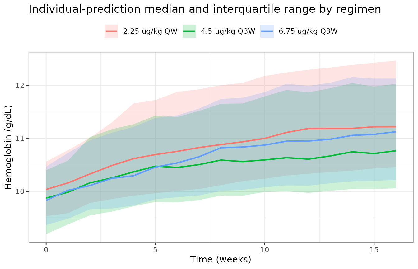

The lag before hemoglobin moves is set by RBCPT = 4.68 days (progenitor maturation) followed by the mature-cell chain, whose transit time is RBCLS = 82.2 days over four compartments. Agoram 2006 notes that 82.2 days is well short of the ~120-day lifespan of healthy adult red cells, consistent with the myelosuppressive effect of chemotherapy and anemia of chronic disease.

Assessment of covariate effects

Agoram 2006’s “Assessment of Effect of Covariates” section predicts the difference in 16-week hemoglobin response, at a fixed 150 ug QW dose (equivalent to the prescribed 2.25 ug/kg QW for a 70 kg patient), between the extremes of each covariate’s range. The published mean (95% CI) is 0.939 (0.283, 1.45) g/dL for body weight and 0.317 (-0.504, 0.877) g/dL for platinum-containing chemotherapy.

cov_events <- function(wt, platin) {
  tibble(
    id = 1L, time = seq(0, 15 * 7, by = 7), amt = 150, evid = 1L, cmt = "depot",
    WT = wt, CONMED_PLATIN = platin, CONMED_PLATIN_GT2 = platin
  ) |>
    dplyr::bind_rows(
      tibble(
        id = 1L, time = seq(0, 16 * 7, by = 7), amt = NA_real_, evid = 0L,
        cmt = "central", WT = wt, CONMED_PLATIN = platin,
        CONMED_PLATIN_GT2 = platin
      )
    ) |>
    dplyr::arrange(time, dplyr::desc(evid))
}

delta_hb <- function(wt, platin) {
  s <- rxode2::rxSolve(
    pd_typical, events = cov_events(wt, platin),
    omega = NA, sigma = NA, returnType = "data.frame"
  ) |>
    dplyr::filter(!is.na(hb))
  s$hb[which.min(abs(s$time - 112))] - s$hb[which.min(abs(s$time - 0))]
}

eff_wt     <- delta_hb(39, 0) - delta_hb(136, 0)
eff_platin <- delta_hb(REF_WT, 0) - delta_hb(REF_WT, 1)

cov_tab <- tibble::tibble(
  Covariate = c("Body weight, 39 kg vs 136 kg", "Platinum chemotherapy, no vs yes"),
  `Published mean (g/dL)` = c(0.939, 0.317),
  `Published 95% CI` = c("(0.283, 1.45)", "(-0.504, 0.877)"),
  `Typical-value contrast (g/dL)` = c(eff_wt, eff_platin),
  `Inside published CI` = c(
    eff_wt > 0.283 && eff_wt < 1.45,
    eff_platin > -0.504 && eff_platin < 0.877
  )
)
knitr::kable(cov_tab, digits = 3, caption = "16-week hemoglobin response difference at 150 ug QW, at the extremes of each covariate.")

16-week hemoglobin response difference at 150 ug QW, at the extremes of each covariate.
Covariate	Published mean (g/dL)	Published 95% CI	Typical-value contrast (g/dL)	Inside published CI
Body weight, 39 kg vs 136 kg	0.939	(0.283, 1.45)	0.734	TRUE
Platinum chemotherapy, no vs yes	0.317	(-0.504, 0.877)	0.291	TRUE


# Deterministic typical-value contrasts, so this gate is stable. The paper's
# figures are Monte Carlo means over the full-IIV cohort rather than
# typical-value contrasts, which is why the point estimates differ while both
# land inside the published intervals.
stopifnot(all(cov_tab$`Inside published CI`))

Both effects reproduce inside the paper’s own published confidence intervals. The paper’s conclusion follows directly from the width of those intervals: “it was not possible to classify any of the covariates as clinically significant”, and dose adjustment on either covariate is not recommended.

Assumptions and deviations

Residual-error form for hemoglobin. Table 4 reports sigma_2^2 = 0.401 without naming an error model, and Equation 2’s log-transformed exponential form is stated only for the pharmacokinetic observations. It is encoded here as additive, SD = sqrt(0.401) = 0.633 g/dL, which is about 6% of the 9.92 g/dL baseline and matches the roughly +/- 1 g/dL scatter about the line of identity in Figure 3A. A log-scale reading of the same variance would be a 63% CV and would spread individual predictions over roughly 3-34 g/dL, which Figure 3A rules out.
Equations 7 and 8 as printed are mutually inconsistent. Equation 8 defines Stim = (1 + Smax*C_DA/(S50 + C_DA)) – the 1 + is inside the parentheses – while Equation 7 is typeset as dA1/dt = Rin(1 = Stim) - kPT*A1, where 1 = Stim is plainly a typographical error. Under either repair (Rin * Stim with the 1 + inside Stim, or Rin * (1 + Stim) with Stim = Smax*C_DA/(S50+C_DA)) the production term is identical: Rin * (1 + Smax*C_DA/(S50 + C_DA)), saturating at 1 + Smax = 1.437. That is the form encoded, and it is the one the abstract describes as an “incremental maximum stimulation of hemoglobin production [of] 43.7%”. Equation 10 is likewise printed with a left-hand side of dA2/dt where the index range i = 3,4,5 on the right makes clear it is dAi/dt.
Rin is derived, not published. The paper does not print a value for Rin or Kout; only Hb0 and RBCLS are estimated. Rin = Hb0 / RBCLS is the drug-free steady state of the published chain, verified above to hold the baseline to within solver tolerance over a simulated year.
Intercompartmental clearance Q is encoded as fixed(). Its Table 3 row is the only one with both a blank standard-error column and a blank bootstrap column; every parameter the paper estimated has both. The paper does not say in prose that Q was fixed, so this is an inference from the table’s structure. It has no effect on any simulation – fixed() is provenance metadata only – but a reviewer with access to the control stream should confirm it.
V2 and Q carry no IIV, and F carries none either. This follows the paper: “It was not possible to estimate the IIV of Q and V2”, and IIV of F was not estimated because the IV and SC data came from separate patients.
No IIV on RBCPT or Smax. The paper states both explicitly. The consequence, which it also flags, is that the estimated S50 variability probably absorbs Smax variability, so covariate conclusions “may equally apply to both these parameters”.
The abstract’s “steady-state volume of distribution, 3390 mL” is the central volume V1, not Vss. Table 3 labels 3390 mL as theta_V1; Vss = V1 + V2 = 3641 mL. The table is taken as authoritative.
PD covariate distributions in the virtual cohort are assumptions. Body weight is drawn as N(69.9, 16.2) truncated to the published 39-136 kg range (Table 2). The paper never tabulates PCNT, so the proportion of patients on platinum-containing chemotherapy is set to 61%, chosen so that the non-platinum tumor types the paper names as typically platinum-free (breast, and the pancreatic / prostate cases it groups under “other”) are the complement. This affects only the width and position of the Figure 4 band, not any parameter.
The CONMED_PLATIN / CONMED_PLATIN_GT2 pair. Agoram 2006 dichotomises a single underlying count, PCNT, at two different thresholds in the same publication: > 2 for the PK model’s clearance effect (Equation 12) and > 0 for the PD model’s S50 effect (Equation 14). Per the standing count-covariate policy the count is carried as two binary indicator columns rather than as an integer, and a data set supporting both models must provide both. In the virtual cohort above the two coincide, because a patient on a 3-weekly platinum regimen receives more than two cycles inside a 16-week window.
Figure 2C landmarks are digitised. The published panel reports no numeric table, so the five landmark values in the comparison table were read off the log-scale figure and are accurate only to gridline resolution; they are checked with a 25% tolerance.
No published NCA table exists for this paper. The PK section therefore validates the NCA output against closed-form identities the structural model must satisfy (AUC0-inf = Dose/CL for the IV arm, and the SC/IV AUC ratio equalling F) rather than against transcribed reference values.