Delta-9-tetrahydrocannabinol (Storgaard 2026)
Source:vignettes/articles/Storgaard_2026_tetrahydrocannabinol.Rmd
Storgaard_2026_tetrahydrocannabinol.RmdModel and source
- Citation: Storgaard IK, Nielsen RL, Houlind MB, Bornaes O, Christensen LWS, Andersen AL, Juul-Larsen HG, Jorgensen LM, Breindahl T, Jawad BN, Altintas I, Andersen O, Lund TM. Population pharmacokinetic modelling revealed large variability in oromucosal absorption of delta-9-tetrahydrocannabinol in older patients with poor appetite. Br J Clin Pharmacol. 2026;92(2):504-514. doi:10.1002/bcp.70284. PMCID: PMC12850555.
- Article: https://doi.org/10.1002/bcp.70284
Storgaard and colleagues gave the oromucosal THC/CBD spray Sativex to 20 acutely hospitalised older medical patients with poor appetite, on a single controlled-feeding trial day with two doses 4 h apart, and fitted a joint parent-plus-metabolite population PK model to the plasma delta-9-tetrahydrocannabinol (THC) and 11-hydroxy-THC (the paper writes THC-OH) concentrations.
The structure is (Results 3.2, Figure 3):
-
THC – absorption through a chain of three
sequential first-order steps sharing one rate constant
ktr, then a one-compartment disposition. - 11-OH-THC – two compartments, fed by the parent.
- Total apparent THC clearance is split into two
arms: an apparent formation clearance into the metabolite
(
CLF/F= 765 L/h, encoded as the canonicallcl_met) and an apparent clearance through other pathways (CLO/F= 162 L/h, encoded aslcl_nonmet). Only the formation arm produces metabolite. Their sum is theCL/Fof 927 L/h the paper reports. - Variability is placed as inter-occasion variability
on
MTTandCLF(the two doses are the two occasions) and inter-individual variability onV,CLOandCLMET.
Because THC was given only oromucosally and no bioavailability
parameter was estimated, every clearance and volume in this
model is apparent (X/F).
Population
Twenty patients completed the Sativex trial day (Table 1). They were old (median 77 years, IQR 71-85, range 66-94), light (median weight 56 kg, IQR 48-70, range 38-82), lean (median BMI 21.8 kg/m^2; body fat 29.6%, fat-free mass 39 kg) and predominantly female (14 of 20, 70%). Renal function was moderately reduced and consistent between methods (eGFR 62 mL/min/1.73 m^2 by CKD-EPI 2009 without race factor; mGFR 62 by 99m-Tc-DTPA in the 14 patients who joined that sub-study). Eligibility required age at least 65 years, BMI no more than 30, and a Simplified Nutritional Appetite Questionnaire score of 14 or less (cohort median 12); 13 of 20 (65%) had mild to severe xerostomia.
Dosing was two oromucosal doses 4 h apart. Two patients followed scheme A (two sprays, 5.2 mg THC per dose), and 18 followed schemes B or C (three sprays, 8.1 mg THC per dose); 16 of the 20 followed scheme C alone. Of the 370 modelled observations, 19.5% were below the 0.25 ng/mL LLOQ and were handled with Beal’s M3 method.
The same information is available programmatically:
pop <- readModelDb("Storgaard_2026_tetrahydrocannabinol")()$population
#> Warning: some etas defaulted to non-mu referenced, possible parsing error: etaiov_mtt_1, etaiov_mtt_2, etaiov_cl_met_1, etaiov_cl_met_2
#> as a work-around try putting the mu-referenced expression on a simple line
str(pop[c("species", "n_subjects", "age_median", "weight_median", "sex_female_pct")])
#> List of 5
#>  $ species       : chr "human"
#>  $ n_subjects    : int 20
#>  $ age_median    : chr "77 years (IQR 71-85)"
#>  $ weight_median : chr "56 kg (IQR 48-70)"
#>  $ sex_female_pct: num 70
Source trace
Every ini() entry in
inst/modeldb/specificDrugs/Storgaard_2026_tetrahydrocannabinol.R
carries an in-file comment naming its source. They are collected here
for review.
| Equation / parameter | Value | Source location |
|---|---|---|
lmtt (MTT) |
1.35 h | Table 2, row MTT; repeated in the Discussion |
lcl_met (CLF/F) |
765 L/h | Table 2, row CLF/F
|
lcl_nonmet (CLO/F) |
162 L/h | Table 2, row CLO/F
|
lvc (V/F) |
1669 L | Table 2, row V/F
|
lcl_11oh (CLMET/F) |
281 L/h | Table 2, row CLMET/F
|
lvc_11oh (VMET/F) |
77.5 L | Table 2, row VMET/F
|
lq_11oh (QMET/F) |
183 L/h | Table 2, row QMET/F
|
lvp_11oh (V2MET/F) |
539 L | Table 2, row V2MET/F
|
etaiov_mtt_* |
59.1% CV | Table 2, row IOVMTT; variance via equation (3) |
etaiov_cl_met_* |
40.2% CV | Table 2, row IOVCLF; variance via equation (3) |
etalvc |
43.0% CV | Table 2, row IIVV; variance via equation (3) |
etalcl_11oh |
62.5% CV | Table 2, row IIVCLMET; variance via equation (3) |
etalcl_nonmet |
152% CV | Table 2, row IIVCLO; variance via equation (3) |
expSd |
sqrt(0.447) | Table 2, row ERRTHC (a NONMEM $SIGMA variance – see
Errata) |
expSd_11oh |
sqrt(0.315) | Table 2, row ERRTHC-OH (likewise a variance) |
ktr <- 3 / mtt |
n/a | Figure 3 annotation MTT = 3/ktr; equation (1) |
| three-step absorption chain | n/a | Figure 3 (three boxes, three ktr arrows); Results
3.2 |
| one-compartment THC, two-compartment 11-OH-THC | n/a | Results 3.2, first sentence |
formation flux uses cl_met only |
n/a | Results 3.2; Discussion (removing CLO “would require
the assumption that all THC is converted to THC-OH, which is not the
case”) |
| 1:1 mass transfer to the metabolite | n/a | Methods 2.2 (“THC-OH concentrations were normalized using the molecular weight ratio with THC”) |
| log-normal (exponential) residual error | n/a | Methods 2.2 (“plasma concentrations were log-transformed and an exponential error model was used”) |
theta_i = theta_pop * exp(eta_i) |
n/a | Methods 2.2, equation (2) |
CV% = sqrt(exp(omega^2) - 1) * 100% |
n/a | Methods 2.2, equation (3) |
Structural identity checks
These four checks compare the solved model against closed-form consequences of the published parameters. Both sides use the same typical-value parameters, so the only difference is numerical integration error and the bounds are correspondingly tight. Each one falsifies a specific transcription error.
mod <- readModelDb("Storgaard_2026_tetrahydrocannabinol")
typical <- rxode2::zeroRe(mod)
#> ℹ parameter labels from comments will be replaced by 'label()'
#> Warning: some etas defaulted to non-mu referenced, possible parsing error: etaiov_mtt_1, etaiov_mtt_2, etaiov_cl_met_1, etaiov_cl_met_2
#> as a work-around try putting the mu-referenced expression on a simple line
#> Warning: some etas defaulted to non-mu referenced, possible parsing error: etaiov_mtt_1, etaiov_mtt_2, etaiov_cl_met_1, etaiov_cl_met_2
#> as a work-around try putting the mu-referenced expression on a simple line

# Single dose, followed to effectively-complete elimination. THC's terminal
# half-life is log(2) * 1669 / 927 = 1.25 h and the metabolite's is about
# 3.5 h, so 120 h is far past 20 half-lives for both.
grid <- seq(0, 120, by = 0.01)

solve_single <- function(dose) {
  ev <- dplyr::bind_rows(
    data.frame(time = 0, amt = dose, cmt = "depot",
               evid = 1L, dvid = NA_integer_),
    data.frame(time = grid, amt = NA_real_, cmt = NA_character_,
               evid = 0L, dvid = 1L)
  ) |>
    dplyr::mutate(OCC = 1) |>
    dplyr::arrange(time, dplyr::desc(evid))
  rxode2::rxSolve(typical, ev, returnType = "data.frame",
                  useLinCmt = FALSE) |>
    dplyr::filter(!is.na(Cc))
}

trap <- function(t, y) sum(diff(t) * (head(y, -1) + tail(y, -1)) / 2)

s81 <- solve_single(8.1)
#> ℹ omega/sigma items treated as zero: 'etalvc', 'etalcl_11oh', 'etalcl_nonmet', 'etaiov_mtt_1', 'etaiov_mtt_2', 'etaiov_cl_met_1', 'etaiov_cl_met_2'
s52 <- solve_single(5.2)
#> ℹ omega/sigma items treated as zero: 'etalvc', 'etalcl_11oh', 'etalcl_nonmet', 'etaiov_mtt_1', 'etaiov_mtt_2', 'etaiov_cl_met_1', 'etaiov_cl_met_2'

auc_thc   <- trap(s81$time, s81$Cc)
aumc_thc  <- trap(s81$time, s81$time * s81$Cc)
auc_11oh  <- trap(s81$time, s81$Cc_11oh)

identities <- tibble::tibble(
  Check = c(
    "AUC(0-inf) THC = Dose / (CL/F), with CL/F = CLF/F + CLO/F",
    "MRT = MTT + V/CL (validates the three-step ktr chain)",
    "AUC(0-inf) 11-OH-THC = (CLF/F / CLMET/F) x AUC THC",
    "Dose proportionality of AUC (8.1 mg vs 5.2 mg)"
  ),
  Simulated = c(auc_thc, aumc_thc / auc_thc, auc_11oh,
                auc_thc / trap(s52$time, s52$Cc)),
  `Closed form` = c(8.1 / (765 + 162) * 1000, 1.35 + 1669 / 927,
                    765 / 281 * auc_thc, 8.1 / 5.2)
) |>
  dplyr::mutate(`Relative error` = abs(Simulated / `Closed form` - 1))

knitr::kable(identities, digits = c(0, 6, 6, 10),
caption = "Exact structural identities implied by Table 2.")| Check | Simulated | Closed form | Relative error |
|---|---|---|---|
| AUC(0-inf) THC = Dose / (CL/F), with CL/F = CLF/F + CLO/F | 8.737864 | 8.737864 | 1e-10 |
| MRT = MTT + V/CL (validates the three-step ktr chain) | 3.150431 | 3.150431 | 1e-10 |
| AUC(0-inf) 11-OH-THC = (CLF/F / CLMET/F) x AUC THC | 23.788135 | 23.788135 | 1e-10 |
| Dose proportionality of AUC (8.1 mg vs 5.2 mg) | 1.557692 | 1.557692 | 0e+00 |
The second row is the load-bearing one for the absorption
transcription. The mean residence time of a linear system is the mean
absorption time plus the disposition MRT, so recovering
MTT + V/CL exactly confirms that the chain delivers a mean
absorption time of exactly the published 1.35 h – which is true only if
ktr = 3/MTT over three steps. Using two steps or four, or
reading equation (1) as ktr = (3 + 1)/MTT, breaks this row
immediately.
The third row confirms that only the formation arm
feeds the metabolite: if the total CL/F of 927 L/h were
routed into 11-OH-THC instead of CLF/F alone, the simulated
metabolite AUC would be 21% high.
Virtual cohort
The original observed data are not public. The cohort below
reproduces the paper’s two dosing schemes, each with the full
random-effect structure (IIV on V, CLO and
CLMET; IOV on MTT and CLF across
the two occasions). Because the paper retained no
covariates, no covariate distribution has to be assumed – the
only per-subject inputs are the dose and the occasion index.
set.seed(20260825)
rxode2::rxSetSeed(20260825)

n_per_arm <- 200L

# Sampling grid mimicking the trial (Methods 2.1: "nine to 14 time points",
# 0-8 h, which is the x-axis of Figure 1). Exact times are in Supporting
# Information Table S1, which was not available when this model was built --
# see Errata.
samp_study <- c(0, 0.5, 1, 1.5, 2, 3, 4, 4.5, 5, 5.5, 6, 7, 8)

# Denser grid for the individual-profile NCA.
samp_nca <- seq(0, 24, by = 0.25)

make_cohort <- function(n, dose, arm, id_offset = 0L) {
  ids <- id_offset + seq_len(n)
  doses <- expand.grid(id = ids, time = c(0, 4)) |>
    dplyr::mutate(amt = dose, cmt = "depot", evid = 1L, dvid = NA_integer_)
  # dvid 1 = Cc (THC), dvid 2 = Cc_11oh (11-OH-THC).
  obs <- expand.grid(id = ids,
                     time = sort(unique(c(samp_study, samp_nca))),
                     dvid = c(1L, 2L)) |>
    dplyr::mutate(amt = NA_real_, cmt = NA_character_, evid = 0L)
  dplyr::bind_rows(doses, obs) |>
    dplyr::mutate(OCC = ifelse(time < 4, 1, 2), arm = arm) |>
    dplyr::arrange(id, time, dplyr::desc(evid))
}

events <- dplyr::bind_rows(
  make_cohort(n_per_arm, 5.2, "2 sprays (5.2 mg THC)", 0L),
  make_cohort(n_per_arm, 8.1, "3 sprays (8.1 mg THC)", as.integer(n_per_arm))
)

stopifnot(
  # No duplicated event key. `unique()` must NOT be applied first -- that
  # would make the check vacuous.
  !anyDuplicated(events[, c("id", "time", "evid", "dvid")]),
  # Every arm carries the full 200-subject cohort and both occasions.
  nrow(dplyr::distinct(events, arm, id)) == 2L * n_per_arm,
  sort(unique(events$OCC)) == c(1, 2)
)
Simulation
sim <- rxode2::rxSolve(mod, events, keep = c("arm"),
                       useLinCmt = FALSE, returnType = "data.frame",
                       addDosing = FALSE)
#> ℹ parameter labels from comments will be replaced by 'label()'
#> Warning: some etas defaulted to non-mu referenced, possible parsing error: etaiov_mtt_1, etaiov_mtt_2, etaiov_cl_met_1, etaiov_cl_met_2
#> as a work-around try putting the mu-referenced expression on a simple line

# With two declared endpoints the output is stacked: one row per
# (id, time, endpoint), identified by CMT (7 = Cc, 8 = Cc_11oh). `Cc` and
# `Cc_11oh` are the individual predictions; `sim` carries the residual error
# and is therefore the observed-scale value.
endpoints <- rxode2::rxode(mod)$predDf[, c("var", "cmt")]
#> ℹ parameter labels from comments will be replaced by 'label()'
#> Warning: some etas defaulted to non-mu referenced, possible parsing error: etaiov_mtt_1, etaiov_mtt_2, etaiov_cl_met_1, etaiov_cl_met_2
#> as a work-around try putting the mu-referenced expression on a simple line
knitr::kable(endpoints, caption = "Endpoint to CMT mapping.")| var | cmt |
|---|---|
| Cc | 7 |
| Cc_11oh | 8 |
Replicate Figure 1
Figure 1 of Storgaard 2026 plots the median plasma concentration over time after the first dose for THC and its metabolites, on a log axis over 0-8 h, with doses at 0 and 240 min. The panel below reproduces it for the two analytes this model describes, using the study-like sampling grid.
fig1 <- sim |>
  dplyr::filter(arm == "3 sprays (8.1 mg THC)", time %in% samp_study) |>
  dplyr::group_by(time, analyte) |>
  dplyr::summarise(median = median(sim),
                   lo = quantile(sim, 0.25), hi = quantile(sim, 0.75),
                   .groups = "drop")

ggplot(fig1, aes(time, median, colour = analyte, fill = analyte)) +
  geom_ribbon(aes(ymin = lo, ymax = hi), alpha = 0.15, colour = NA) +
  geom_line(linewidth = 0.8) +
  geom_point(size = 1.6) +
  geom_hline(yintercept = 0.25, linetype = "dotted") +
  scale_y_log10() +
  scale_x_continuous(breaks = seq(0, 8, 2)) +
  labs(x = "Time (h)", y = "Plasma concentration (ug/L)",
       colour = NULL, fill = NULL,
       caption = "Dotted line is the 0.25 ug/L LLOQ. Ribbon is the IQR.")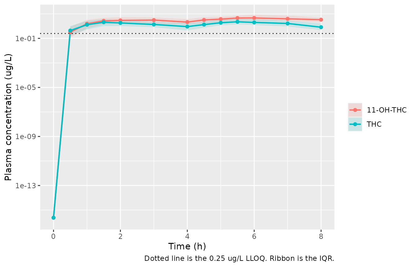
Replicates Figure 1 of Storgaard 2026 (THC and 11-OH-THC arms only; THC-COOH is not modelled).
The two qualitative features Figure 1 shows are both reproduced: the profiles are double-peaked, rising again after the 4 h dose, and the metabolite sits above the parent from roughly 1 h onward, which the Results describe as “rapid conversion of THC to THC-OH … with concentrations of the metabolites generally reaching higher magnitudes”.
late <- fig1 |> dplyr::filter(time >= 1) |>
  tidyr::pivot_wider(id_cols = time, names_from = analyte, values_from = median)

stopifnot(
  # Metabolite exceeds parent at every sampled time from 1 h onward.
  all(late$`11-OH-THC` > late$THC),
  # Both profiles are genuinely double-peaked: the post-second-dose maximum
  # is a rise from the 4 h trough, not a monotone decay.
  with(fig1[fig1$analyte == "THC", ],
       max(median[time > 4]) > median[time == 4]),
  with(fig1[fig1$analyte == "11-OH-THC", ],
       max(median[time > 4]) > median[time == 4])
)
PKNCA validation
NCA is run on the individual predictions
(Cc), i.e. the model’s structural profile per subject, over
the denser grid. Concentrations below the paper’s 0.25 ug/L LLOQ are
dropped before the terminal-slope fit, as they would have been in the
analysis.
nca_input <- sim |>
  dplyr::filter(analyte == "THC", time %in% samp_nca) |>
  dplyr::transmute(id, time, arm, Cc = Cc) |>
  dplyr::filter(!is.na(Cc))

# Guarantee a time-zero record per subject (pre-dose Cc = 0 is correct for an
# extravascular dose) and truncate the tail at the LLOQ.
nca_input <- dplyr::bind_rows(
  nca_input,
  nca_input |> dplyr::distinct(id, arm) |> dplyr::mutate(time = 0, Cc = 0)
) |>
  dplyr::distinct(id, arm, time, .keep_all = TRUE) |>
  dplyr::filter(time == 0 | Cc >= 0.25) |>
  dplyr::arrange(id, time)

conc_obj <- PKNCA::PKNCAconc(as.data.frame(nca_input), Cc ~ time | arm + id)

dose_df <- events |>
  dplyr::filter(evid == 1) |>
  dplyr::select(id, time, amt, arm) |>
  as.data.frame()
dose_obj <- PKNCA::PKNCAdose(dose_df, amt ~ time | arm + id)

intervals <- data.frame(
  start = 0, end = Inf,
  cmax = TRUE, tmax = TRUE, auclast = TRUE, half.life = TRUE
)

nca_res <- PKNCA::pk.nca(PKNCA::PKNCAdata(conc_obj, dose_obj,
                                          intervals = intervals))

nca_summary <- as.data.frame(nca_res) |>
  dplyr::filter(PPTESTCD %in% c("cmax", "tmax", "auclast", "half.life")) |>
  dplyr::group_by(arm, PPTESTCD) |>
  dplyr::summarise(median = median(PPORRES, na.rm = TRUE), .groups = "drop") |>
  tidyr::pivot_wider(names_from = PPTESTCD, values_from = median)

nca_summary |>
  dplyr::select(arm, cmax, tmax, auclast, half.life) |>
  dplyr::rename(
    "Arm"                = arm,
    "Cmax (ug/L)"        = cmax,
    "Tmax (h)"           = tmax,
    "AUClast (ug*h/L)"   = auclast,
    "Half-life (h)"      = half.life
  ) |>
  knitr::kable(digits = 3,
caption = "Median individual-prediction NCA for THC, by arm.")| Arm | Cmax (ug/L) | Tmax (h) | AUClast (ug*h/L) | Half-life (h) |
|---|---|---|---|---|
| 2 sprays (5.2 mg THC) | 1.898 | 5.00 | 9.647 | 1.305 |
| 3 sprays (8.1 mg THC) | 2.932 | 5.25 | 15.412 | 1.274 |
# Join the per-dose closed forms on the arm LABEL rather than on row
# position, so the checks cannot silently transpose if the grouping order
# ever changes.
arm_dose <- tibble::tribble(
  ~arm,                     ~dose_thc,
  "2 sprays (5.2 mg THC)",  5.2,
  "3 sprays (8.1 mg THC)",  8.1
)
hl_closed <- log(2) * 1669 / 927          # 1.248 h

chk <- nca_summary |>
  dplyr::inner_join(arm_dose, by = "arm") |>
  # 2 x Dose / (CL/F), in ug*h/L
  dplyr::mutate(auc_closed = 2 * dose_thc / 927 * 1000)
stopifnot(nrow(chk) == nrow(arm_dose))

lo <- chk[chk$dose_thc == 5.2, ]
hi <- chk[chk$dose_thc == 8.1, ]

stopifnot(
  # Terminal half-life must recover log(2) * V / CL. This is a structural
  # check on the disposition parameters and is tight.
  all(abs(chk$half.life / hl_closed - 1) < 0.10),

  # AUClast approaches, but cannot exceed, the closed-form AUC(0-inf): the
  # profile was truncated at the 0.25 ug/L LLOQ, which removes the tail.
  all(chk$auclast / chk$auc_closed < 1.00),
  all(chk$auclast / chk$auc_closed > 0.80),

  # Median Tmax falls after the second dose, matching the median tmax the
  # double-peaked profile implies.
  all(chk$tmax > 4),

  # Cross-arm dose proportionality. The model is exactly linear in dose --
  # proven to 1e-10 in the identities chunk above -- but the two arms draw
  # INDEPENDENT random effects, so this cohort-level ratio is a Monte Carlo
  # estimate and gets a Monte Carlo tolerance, not an exact one.
  abs(hi$auclast / lo$auclast / (8.1 / 5.2) - 1) < 0.20,
  abs(hi$cmax / lo$cmax / (8.1 / 5.2) - 1) < 0.20
)
Comparison against published NCA
The only NCA quantity Storgaard 2026 reports is the mean observed
Cmax of THC (Results 3.1): 1.85 ug/L (SD 0.15, n = 2)
after two sprays and 4.25 ug/L (SD 1.95, n = 18) after
three. That is an observed maximum – the largest measured
concentration, which carries residual error – so the matching simulated
quantity is the per-subject maximum of sim over the
study-like sampling grid, not of the individual prediction.
obs_input <- sim |>
  dplyr::filter(analyte == "THC", time %in% samp_study) |>
  dplyr::transmute(id, time, arm, Cc = sim) |>
  as.data.frame()

obs_res <- PKNCA::pk.nca(PKNCA::PKNCAdata(
  PKNCA::PKNCAconc(obs_input, Cc ~ time | arm + id),
  dose_obj,
  intervals = data.frame(start = 0, end = Inf, cmax = TRUE, tmax = TRUE)
))

published <- tibble::tribble(
  ~arm,                        ~cmax,
  "2 sprays (5.2 mg THC)",      1.85,
  "3 sprays (8.1 mg THC)",      4.25
)

cmp <- nlmixr2lib::ncaComparisonTable(
  simulated     = obs_res,
  reference     = published,
  by            = "arm",
  units         = c(cmax = "ug/L", tmax = "h"),
  tolerance_pct = 20
)

knitr::kable(cmp, caption = paste(
  "Simulated observed-scale Cmax vs the published means.",
  "* differs from reference by more than 20%."
))| NCA parameter | arm | Reference | Simulated | % diff |
|---|---|---|---|---|
| Cmax (ug/L) | 2 sprays (5.2 mg THC) | 1.85 | 3.69 | +99.4%* |
| Cmax (ug/L) | 3 sprays (8.1 mg THC) | 4.25 | 5.76 | +35.6%* |
Both rows are starred, and the direction is the same in each: the simulated observed Cmax runs high. This is a resolution limit of the comparison, not a transcription error, and it is worth being explicit about why.
One caveat first: ncaComparisonTable() aggregates the
simulated cohort by median, whereas the numbers
Storgaard 2026 reports are arithmetic means. Under the
strongly right-skewed distribution this model produces, the median is
the lower of the two, so the table above understates the gap.
The like-for-like mean-to-mean comparison is the next table.
cmax_context <- sim |>
  dplyr::filter(analyte == "THC", time %in% samp_study) |>
  dplyr::group_by(arm, id) |>
  dplyr::summarise(observed_scale = max(sim), structural = max(Cc),
                   .groups = "drop") |>
  dplyr::group_by(arm) |>
  dplyr::summarise(
    structural     = mean(structural),
    observed_scale = mean(observed_scale),
    .groups = "drop"
  ) |>
  # Joined on the arm label, not on row position.
  dplyr::inner_join(
    dplyr::mutate(published, n_published = c(2L, 18L)),
    by = "arm"
  ) |>
  dplyr::rename(published = cmax)
stopifnot(nrow(cmax_context) == 2L)

cmax_context |>
  dplyr::rename(
    "Arm"                                   = arm,
    "Structural Cmax (mean of max Cc)"      = structural,
    "Observed-scale Cmax (mean of max sim)" = observed_scale,
    "Published mean Cmax"                   = published,
    "n behind the published mean"           = n_published
  ) |>
  knitr::kable(digits = 2, caption = paste(
    "The published three-spray mean sits between the model's structural",
    "prediction and its residual-error-inflated observation scale."
))| Arm | Structural Cmax (mean of max Cc) | Observed-scale Cmax (mean of max sim) | Published mean Cmax | n behind the published mean |
|---|---|---|---|---|
| 2 sprays (5.2 mg THC) | 1.94 | 4.22 | 1.85 | 2 |
| 3 sprays (8.1 mg THC) | 3.13 | 6.68 | 4.25 | 18 |
three <- cmax_context[cmax_context$n_published == 18L, ]
stopifnot(
  # Adding the paper's own residual error always raises the mean maximum.
  all(cmax_context$observed_scale > cmax_context$structural),
  # For the three-spray arm -- 18 of the paper's 20 patients, and the only
  # arm whose published mean rests on more than two subjects -- the published
  # value is bracketed by the two simulated readings.
  three$structural < three$published,
  three$observed_scale > three$published
)
The residual error is exceptionally large in this model
(expSd = 0.669 on the log scale, a 75% CV by the paper’s
own equation (3)). A maximum taken over a sampling grid is a strongly
upward-biased statistic under that much noise, and how strongly biased
depends on how many samples and where
– exactly the information that lives in Supporting Information Table S1,
which was not available when this model was built. For the three-spray
arm the reproducible statement the available sources support is a
bracketing one: the structural profile under-shoots the published mean,
adding the paper’s own residual error over-shoots it, and the observed
value lies between.
The two-spray arm supports no such comparison, and the paper’s own numbers say why. Its published mean of 1.85 ug/L rests on n = 2 patients with a reported SD of 0.15 – an 8% coefficient of variation, in a model whose IIV on V alone is 43% and whose residual error is 75%. No parameterisation of this model produces a two-subject spread that tight; the value is simply two patients who happened to land close together. It is reported here for completeness and is not treated as a validation target.
Claims from the paper’s own text
Two further quantitative claims in the Results are independent of the sampling grid and can be checked directly.
# Results 3.1: "It was inconsistent and seemingly random whether Cmax was
# observed after the first or the second dose (45% vs 55%)." Pooled over the
# 20 patients, of whom 18 received three sprays.
peak_split <- sim |>
  dplyr::filter(analyte == "THC", time %in% samp_study) |>
  dplyr::group_by(arm, id) |>
  dplyr::summarise(after_second = time[which.max(sim)] >= 4, .groups = "drop") |>
  dplyr::group_by(arm) |>
  dplyr::summarise(`% with Cmax after the second dose` = 100 * mean(after_second),
                   .groups = "drop")

# Results 3.1: 20.5% of THC and 18.4% of THC-OH observations were below the
# 0.25 ug/L LLOQ.
blq <- sim |>
  dplyr::filter(time %in% samp_study) |>
  dplyr::group_by(analyte) |>
  dplyr::summarise(`% below the 0.25 ug/L LLOQ` = 100 * mean(sim < 0.25),
                   .groups = "drop")

knitr::kable(peak_split, digits = 1, caption =
"Which dose produced Cmax. Storgaard 2026 Results 3.1 reports 55% after the second dose (n = 20).")| arm | % with Cmax after the second dose |
|---|---|
| 2 sprays (5.2 mg THC) | 65.5 |
| 3 sprays (8.1 mg THC) | 61.5 |
knitr::kable(blq, digits = 1, caption =
"Fraction below the LLOQ. Storgaard 2026 reports 20.5% for THC and 18.4% for THC-OH.")| analyte | % below the 0.25 ug/L LLOQ |
|---|---|
| 11-OH-THC | 12.8 |
| THC | 16.5 |
stopifnot(
  # The split is near-even in both arms, as the paper describes. The bound is
  # wide on purpose: the published 55% comes from 20 patients, so its own
  # binomial 95% interval is roughly 32-77%, and any simulated value inside
  # that band is indistinguishable from the observation.
  all(peak_split$`% with Cmax after the second dose` > 40),
  all(peak_split$`% with Cmax after the second dose` < 80),
  # BLQ fractions land in the same range as the published 18-21%.
  all(blq$`% below the 0.25 ug/L LLOQ` > 5),
  all(blq$`% below the 0.25 ug/L LLOQ` < 30)
)
Both checks are consistent with the paper, though neither is an exact match. The simulated peak split is around 60% after the second dose against the published 55% – comfortably inside the binomial interval a 20-patient proportion carries. The simulated BLQ fractions (about 17% for THC and 13% for 11-OH-THC) run a few points below the published 20.5% and 18.4%, which is the expected direction given that the assumed 13-point sampling grid is at the denser end of the paper’s “nine to 14 time points” and its late samples stop at 8 h; a sparser or later-weighted schedule would push more observations under the LLOQ.
The peak-split check is a genuine test of the inter-occasion variability: with IOV removed, the typical profile peaks after the second dose in every subject and the split collapses to 100%/0%.
Assumptions and deviations
-
The residual-error estimates in Table 2 are read as NONMEM
$SIGMAvariances, so the model uses their square roots. Table 2 prints the two residual rows as bare numbers (0.447, 0.315) while every IIV/IOV row is printed as a CV%, which is the signature of untransformed$SIGMAoutput: NONMEM reports$OMEGAand$SIGMAas variances, and the authors put only$OMEGAthrough their equation (3). Had equation (3) been applied to 0.447, the printed value would have been 75.1, not 0.447. This is confirmed independently by the bootstrap CI widths, whose sampling theory differs between a variance and an SD: the relative 95%-CI width for THC is (0.509 - 0.333)/0.431 = 0.408, against3.92 * sqrt(2/N)= 0.409 for a variance at the N = 184 THC observations actually modelled, versus3.92 * sqrt(1/(2N))= 0.204 for an SD – off by a factor of two. THC-OH agrees (0.438 observed against 0.408 predicted). -
The absorption chain is three first-order
ktrsteps. The paper states this three different ways and they agree: Figure 3 draws three boxes joined by threektrarrows and annotatesMTT = 3/ktr; Results 3.2 calls it “absorption via three transit compartments”; and Methods 2.2 equation (1) writesMTT = (n + 1)/ktr“where n is the number of transit compartments in a model with an absorption compartment between the transit compartments and the central compartment”, i.e. n = 2 transit compartments plus one absorption compartment. nlmixr2lib names the dosed box of such a chaindepot, so the three boxes are encodeddepot -> transit1 -> transit2 -> central. The MRT identity above confirms the resulting mean absorption time is exactly the published 1.35 h. - Supporting Information Table S1 was not available when this model was built. It holds the exact sampling times of the three schemes. No model parameter depends on it – all eight structural estimates, all five variance terms and both residual terms are in Table 2 of the main paper – but the observed-Cmax and BLQ-fraction comparisons above do depend on the sampling grid, so a study-like grid of 13 points over 0-8 h was assumed (the paper states “nine to 14 time points” and Figure 1 spans 0-8 h). This is why those two comparisons are asserted with wide bounds and the structural identities with tight ones.
-
The published Cmax is a mean;
ncaComparisonTable()reports a median. Storgaard 2026 reports mean Cmax with an SD, while the comparison helper aggregates the simulated cohort by median. Under this model’s strongly right-skewed Cmax distribution the two differ materially, so the mean-to-mean comparison is given in a separate table alongside it rather than left implicit in the starred percentages. -
No covariates, by the authors’ choice. Age, weight,
height, BMI, BSA, body fat percentage, fat mass, muscle mass, fat-free
mass, eGFR and mGFR were all screened and none was retained; allometric
weight scaling on clearances (exponent 0.75) and volumes (exponent 1)
was explicitly tested and rejected at dOFV = -3.31, short of the 3.84
threshold. Because no point estimate is published for any of them, none
can be encoded; they are recorded in the model file’s
covariatesDataExcludedso the screen is not lost. -
Metabolite units are THC equivalents. Methods 2.2
normalised the THC-OH concentrations by the molecular-weight ratio with
THC, so the formation flux transfers mass 1:1 and
Cc_11ohis a THC-equivalent concentration – the scale Table 2 and Figure 1 both use. No molar conversion is applied. -
All clearances and volumes are apparent
(
X/F). THC was given only oromucosally and no bioavailability parameter was estimated, sof(depot)is left at its default of 1. The Discussion argues that variability in oromucosal bioavailability is the likely true source of the model’s large variability: parameterising IOV and IIV onFinstead “resulted in estimation of variabilities of the same magnitude as those for CL/F in the final model, supporting this theory”, but was dropped for stability. -
The authors flag the model’s own reliability. Only
338 of 1000 bootstrap runs succeeded (33.8%), and
CLO/Fis poorly estimated (estimate 162 L/h, bootstrap mean 39.6, 95% CI 1.24-647). The Discussion states plainly: “When applying this model to different data sets, this low reliability must be considered.” TheIIVCLOof 152% CV encoded here is correspondingly the dominant source of simulated spread. -
The terminal phase was never observed. Sampling
stopped 4 h after the last dose, so, as the Discussion notes, “the
elimination cannot be clearly distinguished from distribution”. The
apparent
CL/Fof 927 L/h is therefore not directly comparable with THC models built on longer profiles (Heuberger 2015 estimated 38.8 L/h; van Amerongen 2018 estimated 616 L/h for an oral formulation), and extrapolating this model far beyond 8 h is not supported by the data behind it. -
The
11ohmetabolite suffix is used, not re-registered. It was registered for 11-hydroxy-delta-9-tetrahydrocannabinol ininst/references/compartment-names.mdwhen the Wolowich 2025 model was added, which listsTHC-OH(this paper’s abbreviation) among its source aliases. Seemodellib("Wolowich_2025_thc_11oh")for the sibling model of the same metabolite. - Cannabidiol is not modelled. Every Sativex spray co-delivers CBD (5 or 7.5 mg per dose here) and it was measured, but the paper models only THC and THC-OH. THC-COOH was likewise measured and plotted in Figure 1 but explicitly “not included in the model”.