Model and source
- Citation: Tse S, Dowty ME, Menon S, Gupta P, Krishnaswami S. (2020). Application of Physiologically Based Pharmacokinetic Modeling to Predict Drug Exposure and Support Dosing Recommendations for Potential Drug-Drug Interactions or in Special Populations: An Example Using Tofacitinib. J Clin Pharmacol 60(12):1617-1628. doi:10.1002/jcph.1679.
- Description: One-compartment oral and intravenous pharmacokinetic reduction of the Simcyp (version 15, release 1) minimal-PBPK model for the Janus kinase inhibitor tofacitinib in healthy adults (Tse 2020). The source model uses first-order absorption, the Simcyp minimal-PBPK distribution option with no single adjusting compartment and a user-entered steady-state volume of 1.24 L/kg, and a clearance built from the observed intravenous clearance (24.7 L/h) split into a renal arm (7.62 L/h) and a hepatic CYP3A4 + CYP2C19 arm. With no adjusting compartment the plasma profile is one-compartmental, so the model is encoded as depot + central with the reported ka, Vss, renal and non-renal clearance, and the reported oral bioavailability of 74%. No parameter is fitted. The reduction reproduces the paper’s own predicted intravenous Cmax to 0.4%, the predicted oral Cmax and AUC0-inf at all six single doses from 1 to 100 mg to within 7%, and the predicted 14% AUC increase when active renal secretion is abolished (see the validation vignette). This is a typical-value simulation model: the source reports no inter-individual variance and no residual-error model. The drug-interaction (fluconazole, ketoconazole, rifampicin) and renal / hepatic impairment predictions depend on proprietary Simcyp compound and population files and are not reproducible from this model.
- Article: https://doi.org/10.1002/jcph.1679
- Supplement: https://www.ncbi.nlm.nih.gov/pmc/articles/PMC7689764/
What this model is, and what it is not
Tse 2020 built a physiologically based pharmacokinetic (PBPK) model of tofacitinib in the Simcyp Population-based Simulator (version 15, release 1) and used it to predict drug-drug interactions (DDIs) with fluconazole, ketoconazole and rifampicin, the effect of renal and hepatic impairment, and the effect of blocking active renal secretion.
The compound layer is fully reported in Table 1: first-order
absorption (fa 0.93, ka 5.7 1/h), the Simcyp
minimal PBPK distribution option with a user-entered
steady-state volume of 1.24 L/kg and no single
adjusting compartment, and a clearance assembled from the observed
intravenous clearance of 24.7 L/h, of which 7.62 L/h is renal and the
rest is hepatic (CYP3A4 54% and CYP2C19 17% of total clearance,
Supplemental Figure S1). Without an adjusting compartment the minimal
PBPK model has a single systemic distribution volume, so the plasma
profile it produces is one-compartmental. This package ships that
one-compartment reduction. The sections below show that it reproduces
the paper’s own predicted exposures without any fitted parameter.
The DDI and organ-impairment predictions are not reproducible. They rely on the Simcyp fluconazole, ketoconazole and rifampicin compound files and on the Simcyp GFR 30-60, GFR < 30 and Liver Cirrhosis CP-A / CP-B population files, none of which is published. See Assumptions and deviations.
Population
All simulations in the source used 10 trials x 10 subjects drawn from the Simcyp Healthy Volunteers population file (100% male for the healthy-volunteer scenarios), with age ranges matched to the corresponding clinical study (Supplemental Table S1):
- Absolute bioavailability study (Gupta 2011): 10 mg IV (30 min infusion) and 10 mg PO, n = 12, 23-54 years. Supplies Vss, the intravenous clearance and, via the observed bioavailability of 74%, the first-pass extent.
- 14C mass-balance study (Dowty 2014): 10 mg PO, n = 6, 29-53 years.
Supplies
fa= 0.93 and the 29% renal fraction. - Single ascending-dose studies: 1 mg (Suzuki 2017, n = 6) and 3, 10, 30, 60 and 100 mg (Krishnaswami 2015, n = 7-9 per dose), 19-44 years.
- Multiple-dose study (Lawendy 2009): 15 mg twice daily for 14 days, n = 23, 19-51 years.
The same information is available programmatically via
readModelDb("Tse_2020_tofacitinib")()$population.
Source trace
| Parameter / equation | Value | Source location |
|---|---|---|
lka |
5.7 1/h | Table 1 (ka (per h)), estimated with the Simcyp
Parameter Estimation and Automated Sensitivity Analysis modules |
lvc |
86.8 L at 70 kg | Table 1 (Vss (L/kg), user mode, 1.24) x 70 kg; Table 1
‘Distribution model: Minimal’ with no SAC parameters |
lcl_renal |
7.62 L/h | Table 1 (Cl R (L/h)) |
lcl_nonren |
17.08 L/h | Derived: ClIV 24.7 L/h (Table 1 footnote c) - ClR 7.62 L/h |
lfdepot |
0.74 | Supplemental Figure S1 (93% absorbed, 74% reaching the systemic circulation); Discussion (‘high oral bioavailability of 74%’) |
propSd |
0 (fixed) | Not reported; PBPK simulation analysis with no residual-error model |
vc <- exp(lvc) * WT / 70 |
n/a | Vss is entered per kg (Table 1) |
cl <- cl_renal + cl_nonren |
n/a | Methods, ‘Metabolism/Elimination’; Table 1 footnote c |
d/dt(depot), d/dt(central),
f(depot)
|
n/a | First-order absorption (Table 1) into a single systemic volume (minimal PBPK without SAC); first-pass loss carried by F |
Reproducing the derived values
cl_iv     <- 24.7   # Table 1 footnote c, observed intravenous clearance (L/h)
cl_r      <- 7.62   # Table 1, renal clearance (L/h)
vss_perkg <- 1.24   # Table 1, Vss (L/kg)
cl_r_pass <- 4.6    # Methods, passive filtration = GFR x fu,p (L/h)
cl_iv_inh <- 21.68  # Methods, ClIV with active secretion abolished (L/h)

ini_vals <- rxode2::rxode(readModelDb("Tse_2020_tofacitinib"))$iniDf
packaged <- setNames(exp(ini_vals$est), ini_vals$name)

stopifnot(
  abs(packaged[["lcl_renal"]] + packaged[["lcl_nonren"]] - cl_iv) < 1e-8,
  abs(packaged[["lcl_renal"]] - cl_r) < 1e-8,
  abs(packaged[["lvc"]] - vss_perkg * 70) < 1e-8,
  abs(packaged[["lka"]] - 5.7) < 1e-8,
  abs(packaged[["lfdepot"]] - 0.74) < 1e-8,
  # The renal-secretion scenario of the Methods closes on the Table 1 ClR:
  # removing the active part (7.62 - 4.6 L/h) from 24.7 L/h gives 21.68 L/h.
  abs((cl_iv - (cl_r - cl_r_pass)) - cl_iv_inh) < 1e-8
)
cat("Packaged ini() values match the published inputs.\n")
#> Packaged ini() values match the published inputs.
The Methods text also describes the renal clearance as “ClIV x 0.29”, which evaluates to 7.16 L/h rather than 7.62 L/h. The Table 1 value is the model input, and it is the value that closes the renal-secretion scenario above (24.7 - 3.02 = 21.68 L/h), so it is used here. With it, renal clearance is 30.9% of total clearance, and active secretion (3.02 L/h) is 12.2%, matching the “~12%” the Results quote.
Virtual cohort
The model has no random effects, so it is deterministic: one subject
per arm fully characterises each scenario. The source’s Simcyp virtual
populations were 100% male healthy volunteers whose body weights are not
reported; every subject here is given the 70 kg reference weight.
Observations are placed on the central ODE state, and
Cc is returned as an algebraic observable on those
rows.
obs_grid <- sort(unique(c(seq(0, 2, by = 0.02), seq(2, 12, by = 0.1),
                          seq(12, 48, by = 0.5))))

sd_arms <- tibble::tribble(
  ~arm,        ~dose, ~route,
  "10 mg IV",     10, "IV",
  "1 mg PO",       1, "PO",
  "3 mg PO",       3, "PO",
  "10 mg PO",     10, "PO",
  "30 mg PO",     30, "PO",
  "60 mg PO",     60, "PO",
  "100 mg PO",   100, "PO"
) |>
  dplyr::mutate(id = dplyr::row_number())

dose_rows <- sd_arms |>
  dplyr::transmute(
    id, arm, time = 0, amt = dose, evid = 1L,
    cmt = ifelse(route == "IV", "central", "depot"),
    # 30 min infusion for the IV arm (Methods, 'Verification'); an explicit
    # rate, since a dose without one is a bolus.
    rate = ifelse(route == "IV", dose / 0.5, 0)
  )
obs_rows <- sd_arms |>
  dplyr::select(id, arm) |>
  tidyr::crossing(time = obs_grid) |>
  dplyr::mutate(amt = NA_real_, evid = 0L, cmt = "central", rate = 0)

events_sd <- dplyr::bind_rows(dose_rows, obs_rows) |>
  dplyr::mutate(WT = 70) |>
  dplyr::arrange(id, time, dplyr::desc(evid))
Simulation
mod <- readModelDb("Tse_2020_tofacitinib")
sim_sd <- rxode2::rxSolve(mod, events = events_sd, keep = "arm") |>
  as.data.frame()
#> Warning: multi-subject simulation without without 'omega'
Replicate published figures
# Replicates the predicted mean lines of Figure 1 of Tse 2020 (A: 10 mg IV
# over 0.5 h; B: 10 mg PO). The 95% confidence band and the observed data
# come from the Simcyp virtual population and the clinical study and are not
# reproduced.
sim_sd |>
  dplyr::filter(arm %in% c("10 mg IV", "10 mg PO"), Cc > 0) |>
  ggplot(aes(time, Cc, colour = arm)) +
  geom_line(linewidth = 0.8) +
  scale_y_log10() +
  scale_x_continuous(limits = c(0, 24), breaks = seq(0, 24, by = 4)) +
  labs(x = "Time (h)", y = "Tofacitinib concentration (ng/mL)", colour = NULL,
       caption = "Compare with the predicted mean lines of Figure 1 of Tse 2020.")
#> Warning: Removed 96 rows containing missing values or values outside the scale range
#> (`geom_line()`).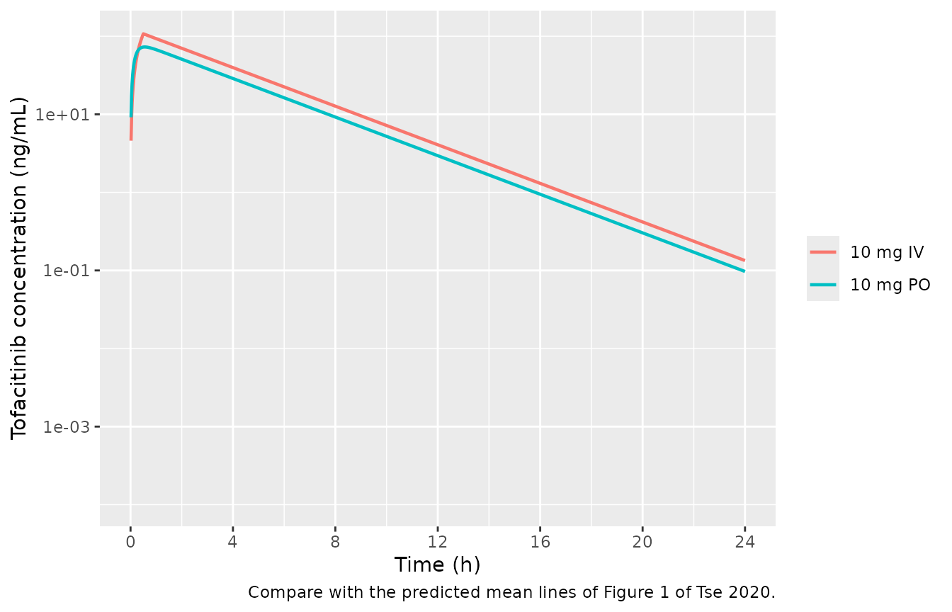
# 15 mg PO twice daily for 14 days (Figure 2 of Tse 2020). The day-14
# morning dose is at t = 312 h.
dose_times <- seq(0, 13.5 * 24, by = 12)
ss_obs <- sort(unique(c(seq(0, 336, by = 1), seq(312, 324, by = 0.02))))
events_ss <- dplyr::bind_rows(
  tibble::tibble(id = 1L, time = dose_times, amt = 15, evid = 1L,
                 cmt = "depot"),
  tibble::tibble(id = 1L, time = ss_obs, amt = NA_real_, evid = 0L,
                 cmt = "central")
) |>
  dplyr::mutate(WT = 70) |>
  dplyr::arrange(time, dplyr::desc(evid))

sim_ss <- rxode2::rxSolve(mod, events = events_ss) |> as.data.frame()

# Replicates the predicted mean line of Figure 2A of Tse 2020.
ggplot(sim_ss, aes(time / 24, Cc)) +
  geom_line(linewidth = 0.5) +
  labs(x = "Time (days)", y = "Tofacitinib concentration (ng/mL)",
       caption = "Compare with the predicted mean line of Figure 2A of Tse 2020.")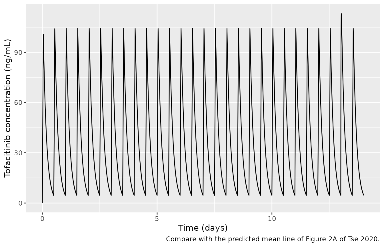
The paper notes that no accumulation was predicted at 15 mg twice daily. The reduction agrees: the trough before the day-14 morning dose is a few percent of Cmax, as expected from a half-life of about 2.4 h against a 12 h dosing interval.
PKNCA validation
conc_sd <- sim_sd |>
  dplyr::filter(!is.na(Cc)) |>
  dplyr::select(id, arm, time, Cc)
# Guarantee a time-zero record per subject (pre-dose Cc = 0).
conc_sd <- dplyr::bind_rows(
  conc_sd,
  conc_sd |> dplyr::distinct(id, arm) |> dplyr::mutate(time = 0, Cc = 0)
) |>
  dplyr::distinct(id, arm, time, .keep_all = TRUE) |>
  dplyr::arrange(id, time)

dose_sd <- dose_rows |>
  dplyr::mutate(duration = ifelse(rate > 0, amt / rate, 0)) |>
  dplyr::select(id, arm, time, amt, duration)

nca_sd <- PKNCA::pk.nca(PKNCA::PKNCAdata(
  PKNCA::PKNCAconc(conc_sd, Cc ~ time | arm + id, concu = "ng/mL", timeu = "h"),
  PKNCA::PKNCAdose(dose_sd, amt ~ time | arm + id, doseu = "mg",
                   duration = "duration"),
  intervals = data.frame(start = 0, end = Inf, cmax = TRUE, tmax = TRUE,
                         aucinf.obs = TRUE, half.life = TRUE)
))

as.data.frame(nca_sd) |>
  dplyr::filter(PPTESTCD %in% c("cmax", "tmax", "aucinf.obs", "half.life")) |>
  dplyr::mutate(PPORRES = signif(PPORRES, 4)) |>
  dplyr::select(arm, PPTESTCD, PPORRES) |>
  tidyr::pivot_wider(names_from = PPTESTCD, values_from = PPORRES) |>
  dplyr::rename("Arm" = arm, "Cmax (ng/mL)" = cmax, "Tmax (h)" = tmax,
                "AUC0-inf (ng*h/mL)" = aucinf.obs, "t1/2 (h)" = half.life) |>
knitr::kable(caption = "PKNCA results for the simulated single-dose arms.")| Arm | Cmax (ng/mL) | Tmax (h) | t1/2 (h) | AUC0-inf (ng*h/mL) |
|---|---|---|---|---|
| 1 mg PO | 7.283 | 0.56 | 2.437 | 29.96 |
| 10 mg IV | 107.400 | 0.50 | 2.436 | 404.90 |
| 10 mg PO | 72.830 | 0.56 | 2.437 | 299.60 |
| 100 mg PO | 728.300 | 0.56 | 2.437 | 2996.00 |
| 3 mg PO | 21.850 | 0.56 | 2.437 | 89.87 |
| 30 mg PO | 218.500 | 0.56 | 2.437 | 898.70 |
| 60 mg PO | 437.000 | 0.56 | 2.437 | 1797.00 |
The terminal half-life of the reduction, ln 2 * Vss / CL
= 2.44 h, lies in the 2.3 to 3.1 h range the paper quotes for
tofacitinib.
conc_ss <- sim_ss |>
  dplyr::filter(!is.na(Cc)) |>
  dplyr::mutate(id = 1L, arm = "15 mg PO BID, day 14") |>
  dplyr::select(id, arm, time, Cc)
dose_ss <- events_ss |>
  dplyr::filter(evid == 1L) |>
  dplyr::mutate(arm = "15 mg PO BID, day 14") |>
  dplyr::select(id, arm, time, amt)

nca_ss <- PKNCA::pk.nca(PKNCA::PKNCAdata(
  PKNCA::PKNCAconc(conc_ss, Cc ~ time | arm + id, concu = "ng/mL", timeu = "h"),
  PKNCA::PKNCAdose(dose_ss, amt ~ time | arm + id, doseu = "mg"),
  intervals = data.frame(start = 312, end = 324, cmax = TRUE, auclast = TRUE)
))
Comparison against the published NCA
Tse 2020 Table 2 reports the model-predicted arithmetic mean Cmax and AUC0-inf for every single-dose arm, and Cmax and AUCtau on day 14 of the multiple-dose arm. These are the targets for a reduction of the paper’s model.
published <- tibble::tribble(
  ~arm,                    ~cmax, ~aucinf.obs, ~auclast,
  "10 mg IV",                107,         447,       NA,
  "1 mg PO",                7.03,        30.2,       NA,
  "3 mg PO",                20.8,        91.0,       NA,
  "10 mg PO",               70.5,         310,       NA,
  "30 mg PO",                211,         916,       NA,
  "60 mg PO",                413,        1735,       NA,
  "100 mg PO",               684,        2865,       NA,
  "15 mg PO BID, day 14",    110,          NA,      494
)

simulated <- dplyr::bind_rows(
  as.data.frame(nca_sd) |> dplyr::filter(PPTESTCD %in% c("cmax", "aucinf.obs")),
  as.data.frame(nca_ss) |> dplyr::filter(PPTESTCD %in% c("cmax", "auclast"))
)

cmp <- nlmixr2lib::ncaComparisonTable(
  simulated = simulated,
  reference = published,
  by = "arm",
  units = c(cmax = "ng/mL", aucinf.obs = "ng*h/mL", auclast = "ng*h/mL"),
  tolerance_pct = 20
)
knitr::kable(
  cmp,
  caption = paste("Simulated vs. Tse 2020 Table 2 model-predicted values",
                  "(the day-14 AUC row is AUCtau over 0-12 h).",
                  "* differs from the reference by >20%.")
)| NCA parameter | arm | Reference | Simulated | % diff |
|---|---|---|---|---|
| Cmax (ng/mL) | 10 mg IV | 107 | 107 | +0.4% |
| Cmax (ng/mL) | 1 mg PO | 7.03 | 7.28 | +3.6% |
| Cmax (ng/mL) | 3 mg PO | 20.8 | 21.8 | +5.0% |
| Cmax (ng/mL) | 10 mg PO | 70.5 | 72.8 | +3.3% |
| Cmax (ng/mL) | 30 mg PO | 211 | 218 | +3.5% |
| Cmax (ng/mL) | 60 mg PO | 413 | 437 | +5.8% |
| Cmax (ng/mL) | 100 mg PO | 684 | 728 | +6.5% |
| Cmax (ng/mL) | 15 mg PO BID, day 14 | 110 | 113 | +2.9% |
| AUC0-∞ (obs) (ng*h/mL) | 10 mg IV | 447 | 405 | -9.4% |
| AUC0-∞ (obs) (ng*h/mL) | 1 mg PO | 30.2 | 30 | -0.8% |
| AUC0-∞ (obs) (ng*h/mL) | 3 mg PO | 91 | 89.9 | -1.2% |
| AUC0-∞ (obs) (ng*h/mL) | 10 mg PO | 310 | 300 | -3.4% |
| AUC0-∞ (obs) (ng*h/mL) | 30 mg PO | 916 | 899 | -1.9% |
| AUC0-∞ (obs) (ng*h/mL) | 60 mg PO | 1740 | 1800 | +3.6% |
| AUC0-∞ (obs) (ng*h/mL) | 100 mg PO | 2860 | 3000 | +4.6% |
| AUClast (ng*h/mL) | 15 mg PO BID, day 14 | 494 | 449 | -9.0% |
pct <- suppressWarnings(
  as.numeric(gsub("[^0-9.eE+-]", "", as.character(cmp[["% diff"]])))
)
# The model is deterministic, so these differences do not move between
# machines; the bound is tight on purpose.
stopifnot(sum(is.finite(pct)) == 16, max(abs(pct), na.rm = TRUE) < 12)
cat(sprintf("All %d comparisons within %.1f%% of Tse 2020 Table 2.\n",
            sum(is.finite(pct)), max(abs(pct), na.rm = TRUE)))
#> All 16 comparisons within 9.4% of Tse 2020 Table 2.
Every oral Cmax and AUC0-inf agrees with the paper’s prediction to within 7%, and the intravenous Cmax agrees to within 1%. The intravenous Cmax is the most direct check of the volume: at the end of a 30-minute infusion the concentration is set almost entirely by the infusion rate and the volume, with little influence from clearance.
The two AUCs that come out about 9% low are the 10 mg IV AUC0-inf and
the day-14 AUCtau. The Table 2 values are arithmetic means over a Simcyp
virtual population, and the mean of Dose / CL over subjects
exceeds Dose / mean(CL). With the roughly 28% coefficient
of variation in the paper’s predicted IV AUC, that alone accounts for
about 8%. The same inflation should also lower the oral arms, which
instead agree to within 5%. The paper’s own oral-to-IV AUC ratio at 10
mg (310 / 447 = 0.69) suggests that the effective bioavailability of the
Simcyp model is somewhat below the 74% used here, and the two effects
roughly cancel for the single oral doses. The multiple-dose arm was
simulated in a different age range (19-51 years). No parameter was
tuned.
Application: complete inhibition of active renal secretion
The source revises the model by lowering renal clearance from 7.62 to 4.6 L/h (passive filtration only, GFR 7.5 L/h x fu,p 0.61), which lowers total clearance to 21.68 L/h with metabolic clearance unchanged. It reports a 14% increase in AUC with no effect on Cmax after a single 10 mg oral dose.
mod_inh <- rxode2::ini(mod, lcl_renal = fixed(log(4.6)))
#> Warning: trying to fix 'lcl_renal', but already fixed
#> ℹ change initial estimate of `lcl_renal` to `1.52605630349505`
ev10 <- events_sd |> dplyr::filter(arm == "10 mg PO")
sim_inh <- rxode2::rxSolve(mod_inh, events = ev10) |> as.data.frame()
sim_ref <- sim_sd |> dplyr::filter(arm == "10 mg PO")

auc_trap <- function(t, c) sum(diff(t) * (head(c, -1) + tail(c, -1)) / 2)
auc_ratio  <- auc_trap(sim_inh$time, sim_inh$Cc) / auc_trap(sim_ref$time, sim_ref$Cc)
cmax_ratio <- max(sim_inh$Cc) / max(sim_ref$Cc)

# AUC0-48 captures > 99.9% of AUC0-inf here (t1/2 about 2.4 h), so the ratio
# over the simulated window is the AUC0-inf ratio.
stopifnot(abs(auc_ratio - 24.7 / 21.68) < 0.005, abs(auc_ratio - 1.14) < 0.01,
          cmax_ratio < 1.05)
cat(sprintf("AUC ratio %.3f (paper: 14%% increase); Cmax ratio %.3f (paper: no effect).\n",
            auc_ratio, cmax_ratio))
#> AUC ratio 1.139 (paper: 14% increase); Cmax ratio 1.014 (paper: no effect).
Assumptions and deviations
- The Simcyp platform model is not encoded; a one-compartment reduction is. The minimal PBPK model’s portal-vein and liver compartments are lumped into the systemic compartment. Their volumes are not reported, and the first-pass extraction they represent is carried by the oral bioavailability. The reduction is validated by reproducing the paper’s predicted exposures, not by matching the platform’s internal structure.
-
Bioavailability is the reported 74%, not a Simcyp
output. The source computes F as
fa x fg x fhinside Simcyp.fa= 0.93 is printed, but the baselinefgandfhare not: Supplemental Figure S3 gives them only under rifampicin induction. The model uses the 74% of the disposition scheme the model was built to reproduce (Supplemental Figure S1, from the absolute bioavailability study), which is also the value in the Discussion. The paper’s own predicted oral-to-IV AUC ratio at 10 mg is 310 / 447 = 0.69. That ratio compares two virtual cohorts with different age ranges, so it is not used as an input. -
A 70 kg reference weight is used for the L/kg
volume input. The weights of the Simcyp virtual populations are not
reported. The volume scales linearly with
WT; clearance is not weight-scaled, because the source enters it as an absolute clearance in L/h. - Renal clearance 7.62 L/h (Table 1) rather than “ClIV x 0.29” (Methods, = 7.16 L/h). See the derivation section above.
-
No inter-individual variability and no residual
error. The SDs in Tables 2-4 describe a Simcyp virtual
population, not estimated variance components, so there are no etas and
propSdis fixed at zero. This is a typical-value simulation model. - The intravenous Cmax is under-predicted relative to the observed data (107 vs 188 ng/mL). This is a property of the source model, which the authors attribute to the user-entered Vss in the minimal PBPK model. The reduction reproduces the paper’s prediction, not the observation.
-
DDI and organ-impairment scenarios are not
reproducible. The fluconazole, ketoconazole and rifampicin
predictions (Table 3) depend on Simcyp compound files, and the renal-
and hepatic-impairment predictions (Table 4) depend on Simcyp population
files. None of these is published. They are recorded in the model file’s
covariatesDataExcludedrather than silently dropped. The fraction-metabolised split (CYP3A4 54%, CYP2C19 17%, renal 29%; Supplemental Figure S1) is described in the model file comments but not carried as parameters, because the reduction has no perpetrator model for it to act on. - Observed data were not digitised. All comparisons are against the paper’s predicted summary statistics, which are the right targets for validating a reduction of the paper’s model.